Page 94 - Rapid Learning in Robotics

80 Extensions to the Standard PSOM Algorithm

6.3.1 Approximation Example: The Gaussian Bell

As a first example to illustrate the Local-PSOMs we consider the Gaussian
bell function

x x
x exp (6.1)

with chosen to obtain a “sharply”
curved function in the square

region . Fig. 6.3 shows the situation for a training data set,
Fig. 6.3b, equidistantly sampled on the test function surface plotted in
Fig. 6.3a.

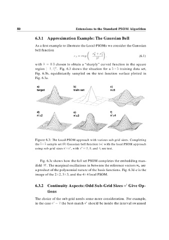
a) b) c)
target train set n=5

d) e) f)

n’=2 n’=3 n’=4

Figure 6.3: The Local-PSOM approach with various sub-grid sizes. Completing
the sample set b Gaussian bell function a with the local PSOM approach

using sub-grid sizes n n , with n and
; see text.

Fig. 6.3c shows how the full set PSOM completes the embedding man-
ifold M. The marginal oscillations in between the reference vectors w a are
a product of the polynomial nature of the basis functions. Fig. 6.3d-e is the
image of the 2 2, 3 3, and the 4 4 local PSOM.

6.3.2 Continuity Aspects: Odd Sub-Grid Sizes n Give Op-

tions

The choice of the sub-grid needs some more consideration. For example,

in the case n the best-match s should be inside the interval swanned