Page 99 - Rapid Learning in Robotics

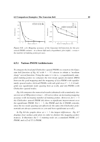
6.5 Comparison Examples: The Gaussian Bell 85

0.3 1
equidistant spacing 2x2
Chebyshev spacing 3x3
0.25 4x4
0.1 equidistant spacing, full set
Chebyshev spacing, full set
Chebyshev spacing, full set
0.2
Deviation (nrms) 0.15 Deviation (nrms) 0.01
0.1
0.001
0.05

0 0.0001
3 4 5 6 8 10 12 3 4 5 6 8 10 12
Number of Knots ^2 Number of Training Knots per Axes
Figure 6.6: a–b; Mapping accuracy of the Gaussian bell function for the pre-
sented PSOM variants – in a linear (left) and a logarithmic plot (right) – versus n
the number of training points per axes.

6.5.1 Various PSOM Architectures

To compare the local and Chebyshev spaced PSOMs we return to the Gaus-
sian bell function of Eq. 6.1 with chosen to obtain a “medium
sharp” curved function. Using the same n n (in x ) x equidistantly sam-
pled training points we compute the root mean square deviation (RMS)
between the goal mapping and the mapping of (i) a PSOM with equidis-

tantly spaced nodes, (ii) local PSOMs with sub-grid sizes n , 3, 4 (sub-
grids use equidistant node spacing here as well), and (iii) PSOMs with
Chebyshev spaced nodes.

Fig. 6.6 compares the numerical results (obtained with a randomly cho-
sen test set of 500 points) versus n. All curves show an increasing mapping
accuracy with increasing number of training points. However, for n
the Chebyshev spaced PSOM (iii) shows a significant improvement over

the equidistant PSOM. For n , the PSOM and the C-PSOM coincide,
since the two node spacings are effectively the same (the Chebyshev poly-
nomials are always symmetric to zero and here equidistant as well.)
In Fig. 6.6 the graphs show at n the largest differences. Fig. 6.7
displays four surface grid plots in order to distinct the mapping perfor-
mances. It illustrates the training node set, a standard PSOM, a C-

PSOM, and a (2-of-5) L-PSOM.