Page 101 - Rapid Learning in Robotics

6.5 Comparison Examples: The Gaussian Bell 87

6.5.2 LLM Based Networks

The following illustrations compare the approximation performance of
discrete Local Linear Maps (LLMs) for the same bell-shaped test function
(note the different scaling).

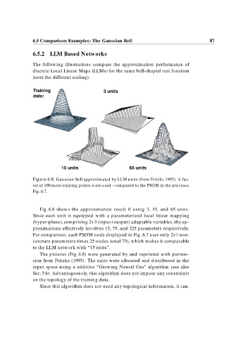
Training 3 units
data:

15 units 65 units

Figure 6.8: Gaussian Bell approximated by LLM units (from Fritzke 1995). A fac-
tor of 100 more training points were used - compared to the PSOM in the previous
Fig. 6.7.

Fig. 6.8 shows the approximation result if using 3, 15, and 65 units.
Since each unit is equipped with a parameterized local linear mapping
(hyper-plane), comprising 2+3 (input+output) adaptable variables, the ap-
proximations effectively involves 15, 75, and 325 parameters respectively.
For comparison, each PSOM node displayed in Fig. 6.7 uses only 2+1 non-
constant parameters times 25 nodes (total 75), which makes it comparable
to the LLM network with “15 units”.
The pictures (Fig. 6.8) were generated by and reprinted with permis-
sion from Fritzke (1995). The units were allocated and distributed in the
input space using a additive “Growing Neural Gas” algorithm (see also
Sec. 3.6). Advantageously, this algorithm does not impose any constraints
on the topology of the training data.
Since this algorithm does not need any topological information, it can-