Page 106 - Rapid Learning in Robotics

92 Extensions to the Standard PSOM Algorithm

R:0.6, f:0.6 R:0.6, f:0.6 (3 3 3 3 -chebyshev)
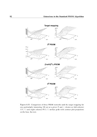
Target mapping
Z phase
1100 100
1000
900
800 50
700
600
500 0
400
300 -50
200
100
0 -100
10 10
0 5 0 5
L[H] 0.5 C[uF] L[H] 0.5 C[uF]
1 1

4
R:0.6, f:0.6 3 PSOM R:0.6, f:0.6 (3 3 3 3 -chebyshev)
1500
Z phase
150
1000
100
50
500
0
-50
0
-100
-150
10 10
-500
0 5 0 5
L[H] 0.5 C[uF] L[H] 0.5 C[uF]
1 1
R:0.6, f:0.6 4 R:0.6, f:0.6 (5 5 5 5 -chebyshev)
(3-of-5) L-PSOM
Z phase
1100 100
1000
900
800 50
700
600 0
500
400
300 -50
200
100
0 -100
10 10
0 0
5 5
0.5 0.5
L[H] C[uF] L[H] C[uF]
1 1
4
R:0.6, f:0.6 5 PSOM R:0.6, f:0.6 (5 5 5 5 -chebyshev)
Z phase
150
1100
1000 100
900
800
700 50
600
500 0
400
300 -50
200
100
0 -100
10 10
0 5 0 5
L[H] 0.5 C[uF] L[H] 0.5 C[uF]
1 1
Figure 6.11: Comparison of three PSOM networks and the target mapping for
one particularly interesting 2 D cut at a given R and f, drawn as (left column)
Z L C and (right column) L C surface grids with contour plot projections
on the base. See text.