Page 98 - Rapid Learning in Robotics

84 Extensions to the Standard PSOM Algorithm

1
0.5
1
-1 -0.5 0.5 1
0.5
s
-0.5 -1 -0.5 0.5 1 2
-0.5
-1 -1
s 1
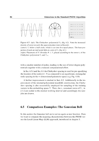
Figure 6.5: (left:) The Chebyshev polynomial T (Eq. 6.2). Note the increased
density of zeros towards the approximation interval bounds .
(center:) T below a half circle, which is cut into five equal pieces. The base pro-
jection of each arc mid point falls at a zero of T (Eq. 6.3.)
(right:) Placement of 5 10 nodes A S, placed according to the zeros a j of the
Chebyshev polynomial T and T .

with a smaller number of nodes, leading to the use of lower-degree poly-
nomials together with a reduced computational effort.
In Sec. 6.5.1 and Sec. 8.1 the Chebyshev spacing is used for pre-specifying
the location of the nodes a A as compared to an equidistant, rectangular
node-spacing in the m-dimensional parameter space (e.g. Fig. 4.10).

A further improvement is studied in Sect. 8.2. Additionally to the im-
provement of the internal polynomial manifold construction, the Cheby-
shev spacing is also successfully employed for sampling of the training
vectors in the embedding space X. Then, the n (constant) zeros of T n in

[-1,1] are scaled to the desired working interval and accordingly the sam-
ples are drawn.

6.5 Comparison Examples: The Gaussian Bell

In this section the Gaussian bell curve serves again as test function. Here
we want to compare the mapping characteristics between the PSOM ver-
sus the Local-Linear-Map (LLM) approach, introduced in chapter 3.