Page 95 - Rapid Learning in Robotics

6.3 The Local-PSOM 81

by the two selected nodes. This requires to shift the selected node window,

if s is outside the interval. This happens e.g. when starting at the best-

match node a , the “wrong” next neighboring node is considered first (left
instead of right).
Fig. 6.3d illustrates that the resulting mapping is continuous – also along
edge connecting reference vectors. Because of the factorization of the basis
functions the polynomials are continuous at the edges, but the derivatives
perpendicular to the edges are not, as seen by the sharp edges. An analo-

gous scheme is also applicable for all higher even numbers of nodes n.
What happens for odd sub-grid sizes? Here, a central node exists and

can be fixated at the search starting location a . The price is that an input,
continuously moving from one reference vector to the next will experience
halfway that the selected sub-grid set changes. In general this results in a
discontinuous associative completion, which can be seen in Fig. 6.3e which
coincides with Fig. 6.4a).

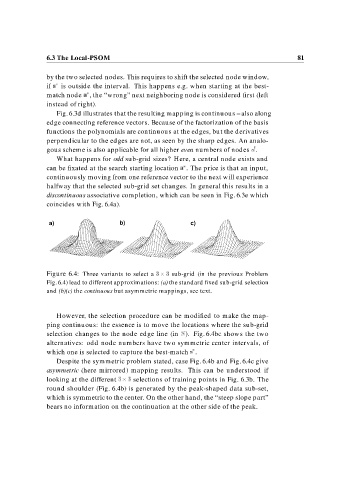
a) b) c)

Figure 6.4: Three variants to select a sub-grid (in the previous Problem
Fig. 6.4) lead to different approximations: (a) the standard fixed sub-grid selection
and (b)(c) the continuous but asymmetric mappings, see text.

However, the selection procedure can be modified to make the map-
ping continuous: the essence is to move the locations where the sub-grid
selection changes to the node edge line (in S). Fig. 6.4bc shows the two
alternatives: odd node numbers have two symmetric center intervals, of

which one is selected to capture the best-match s .
Despite the symmetric problem stated, case Fig. 6.4b and Fig. 6.4c give
asymmetric (here mirrored) mapping results. This can be understood if
looking at the different selections of training points in Fig. 6.3b. The
round shoulder (Fig. 6.4b) is generated by the peak-shaped data sub-set,
which is symmetric to the center. On the other hand, the “steep slope part”
bears no information on the continuation at the other side of the peak.