Page 97 - Reliability and Maintainability of In service Pipelines

86 Reliability and Maintainability of In-Service Pipelines

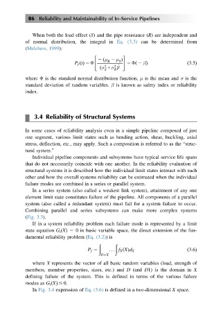
When both the load effect (S) and the pipe resistance (R) are independent and
of normal distribution, the integral in Eq. (3.3) can be determined from
(Melchers, 1999):

" #
P f tðÞ 5 Φ 2 ðμ 2 μ Þ 5 Φ 2 βÞ ð3:5Þ
R
S
ð
1
2
2
ðσ 1σ Þ 2
S R
where Φ is the standard normal distribution function, μ is the mean and σ is the
standard deviation of random variables. β is known as safety index or reliability
index.
3.4 Reliability of Structural Systems

In some cases of reliability analysis even in a simple pipeline composed of just
one segment, various limit states such as bending action, shear, buckling, axial
stress, deflection, etc., may apply. Such a composition is referred to as the “struc-
tural system.”
Individual pipeline components and subsystems have typical service life spans
that do not necessarily coincide with one another. In the reliability evaluation of
structural systems it is described how the individual limit states interact with each
other and how the overall systems reliability can be estimated when the individual
failure modes are combined in a series or parallel system.
In a series system (also called a weakest link system), attainment of any one
element limit state constitutes failure of the pipeline. All components of a parallel
system (also called a redundant system) must fail for a system failure to occur.
Combining parallel and series subsystems can make more complex systems
(Fig. 3.3).
If in a system reliability problem each failure mode is represented by a limit
state equation G i (X) 5 0 in basic variable space, the direct extension of the fun-
damental reliability problem (Eq. (3.2))is
ð ð
P f 5 ... f X ðXÞd X ð3:6Þ
DAX
where X represents the vector of all basic random variables (load, strength of
members, member properties, sizes, etc.) and D (and D1) is the domain in X
defining failure of the system. This is defined in terms of the various failure
modes as G i ðXÞ # 0.
In Fig. 3.4 expression of Eq. (3.6) is defined in a two-dimensional X space.