Page 274 - Renewable Energy Devices and System with Simulations in MATLAB and ANSYS

Design Considerations for Wind Turbine Systems 261

14
12
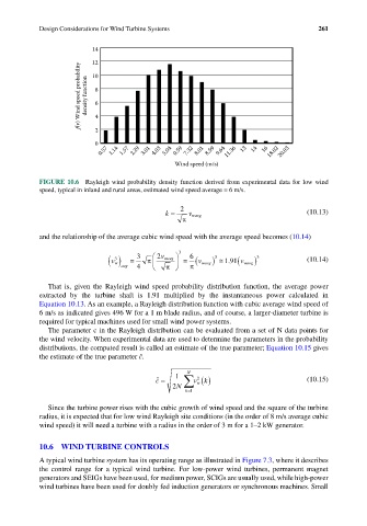
f(v) Wind speed probability density function 8 6 4
10

0 2
0.57 1.14 1.57 2.29 3.01 4.03 5.04 0.59 7.32 8.01 8.59 9.64 11.36 13 14 16 18.02 20.03
Wind speed (m/s)

FIGURE 10.6 Rayleigh wind probability density function derived from experimental data for low wind
speed, typical in inland and rural areas, estimated wind speed average = 6 m/s.

2
k = v wavg (10.13)
π

and the relationship of the average cubic wind speed with the average speed becomes (10.14)

6
v w ( ) = 3 π   2 v wavg   3 = ( v wavg) ≅ . v wavg) 3 (10.14)
191(
3
3
avg 4  π  π
That is, given the Rayleigh wind speed probability distribution function, the average power
extracted by the turbine shaft is 1.91 multiplied by the instantaneous power calculated in
Equation 10.13. As an example, a Rayleigh distribution function with cubic average wind speed of
6 m/s as indicated gives 496 W for a 1 m blade radius, and of course, a larger-diameter turbine is
required for typical machines used for small wind power systems.
The parameter c in the Rayleigh distribution can be evaluated from a set of N data points for
the wind velocity. When experimental data are used to determine the parameters in the probability
distributions, the computed result is called an estimate of the true parameter; Equation 10.15 gives
the estimate of the true parameter ĉ.

1 N
ˆ c = ∑ v w () (10.15)
2
k
2 N
k=1
Since the turbine power rises with the cubic growth of wind speed and the square of the turbine
radius, it is expected that for low wind Rayleigh site conditions (in the order of 8 m/s average cubic
wind speed) it will need a turbine with a radius in the order of 3 m for a 1–2 kW generator.

10.6 WIND TURBINE CONTROLS
A typical wind turbine system has its operating range as illustrated in Figure 7.3, where it describes
the control range for a typical wind turbine. For low-power wind turbines, permanent magnet
generators and SEIGs have been used, for medium power, SCIGs are usually used, while high-power
wind turbines have been used for doubly fed induction generators or synchronous machines. Small