Page 273 - Renewable Energy Devices and System with Simulations in MATLAB and ANSYS

260 Renewable Energy Devices and Systems with Simulations in MATLAB and ANSYS ®
®

ρ
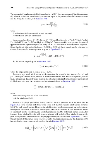
The air density can be corrected by the gas law (ρ= PRT ) for every pressure (P) and temperature
/
(T), where R is the ideal, or universal, gas constant, equal to the product of the Boltzmann constant
and the Avogadro constant, with Equation 10.8.
273 P
.
ρ= 1 2929 (10.8)
T 760
where
P is the atmospheric pressure (in mm of mercury)
T is the Kelvin absolute temperature
ρ
3
Under normal conditions (T = 296 Kand P = 760 mmHg ), the value of is 1.192 kg/m and at
3
.
T = 288K( 15 °C) and P = 760 mmHg it is 1 225kg/m . One can consider a temperature decrease of
approximately one degree centigrade for every 150 m. The influence of humidity can be neglected.
If just the altitude h (in meters) is known (10,000 ft = 3,048 m), the air density can be estimated by
the two first terms of a series expansion as given in Equation 10.9.
 0 297 
.
−  h 
−4
.
.
ρ = ρ 0 e  3048  ≈ 1 225 −1 194 ×10 h (10.9)
So, the turbine torque is given by Equation 10.10.
2
=
T t = P t /ωρ ARv C T /2 (10.10)
W
where the torque coefficient is defined as C T = C p /λ.
2
Suppose a very small wind turbine needs evaluation for a certain site. Assume S = 1 m and
3
.
ρ= 1 2929kg/m , the maximum potential of wind can be obtained from the earlier equation (without
taking into account the aerodynamic losses in the rotor, the wind speed variations at several points of
the blade sweeping area, the rotor type, and so on) as calculated by Equation 10.11.
P = 0 5926 0 6464 × v w = 0 3831. × 3 (10.11)
×
3
.
.
A v w
where
/
2
PA is the wind power per swept area (W/m )
v w is the wind speed (m/s)
Suppose a Rayleigh probability density function such as provided with the wind data in
Figure 10.6. For a constant and steady wind speed of 6 m/s the available shaft turbine power is
260 W for such a small turbine. However, the wind is neither steady nor constant, and such instanta-
neous power calculation is not useful for sizing and for economic studies. In fact, the random nature
of wind must also be considered, and a statistical analysis must be performed. Let us assume, for
instance, that a wind turbine site with strong winds and with periods of low wind and some really
good average speed can be defined as a Rayleigh probability density function. Equation 10.12 shows
the calculation of the average cubic wind speed under Rayleigh conditions, and the shape factor ()k
is related to the cubic average wind speed as given in Equation 10.12.

∞ ∞  2 
v w ( ) avg ∫ v hv dv = ∫ v w ⋅ v 2 2 exp −    v w    dv = 3 3 k 3 π (10.12)
w ()
3
3
=
3
0 0 k    k    4