Page 66 - Reservoir Geomechanics

50 Reservoir geomechanics

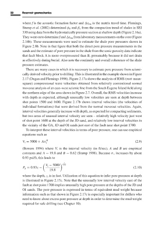
where f is the acoustic formation factor and
t ma is the matrix travel time. Flemings,
Stump et al.(2002) determined φ 0 and β c from the compaction trend of shales in SEI
330 using data from the hydrostatically pressure section at shallow depth (Figure 2.16a).
They went on to determine f and
t ma from laboratory measurements on the core (Figure
2.16b). These measurements were used to estimate the shale pore pressures shown in
Figure 2.8b. Note in that figure that both the direct pore pressure measurements in the
sands and the estimate of pore pressure in the shale from the sonic porosity data indicate
that fault block A is more overpressured than B, presumably because it did not drain
as effectively during burial. Also note the continuity and overall coherence of the shale
pressure estimates.
There are many cases in which it is necessary to estimate pore pressure from seismi-
cally derived velocity prior to drilling. This is illustrated in the example shown in Figure
2.17 (Dugan and Flemings 1998). Figure 2.17a shows the analysis of RMS (root-mean-
square) compressional wave velocities obtained from relatively conventional normal
moveout analysis of an east–west seismic line from the South Eugene Island field along
the northern edge of the area shown in Figure 2.7.Overall, the RMS velocities increase
with depth as expected, although unusually low velocities are seen at depth between
shot points 1500 and 1600. Figure 2.17b shows interval velocities (the velocities of
individual formations) that were derived from the normal moveout velocities. Again,
interval velocities generally increase with depth, as expected for compacting sediments,
buttwo areas of unusual interval velocity are seen – relatively high velocity just west
of shot point 1600 at the depth of the JD sand, and relatively low interval velocities in
the vicinity of the GA, JD and OI sands just east of the fault near shot point 1700.
To interpret these interval velocities in terms of pore pressure, one can use empirical
equations such as

V i = 5000 + Aσ B (2.9)
v
(Bowers 1994) where V i is the interval velocity (in ft/sec), A and B are empirical
constants and A = 19.8 and B = 0.62 (Stump 1998). Because σ v increases by about
0.93 psi/ft, this leads to
1
V i − 5000 0.62

P p = 0.93z − (2.10)
19.8
where the depth, z,isin feet. Utilization of this equation to infer pore pressure at depth
is illustrated in Figure 2.17c. Note that the unusually low interval velocity east of the
fault at shot point 1700 implies unusually high pore pressure at the depths of the JD and
OI sands. The pore pressure is expressed in terms of equivalent mud weight because
information such as that shown in Figure 2.17cis especially important for drillers who
need to know about excess pore pressure at depth in order to determine the mud weight
required for safe drilling (see Chapter 10).