
Page 199 -
P. 199
182 Computed-Torque Control
A simple time response program, TRESP, is given in Appendix B. Given a
subroutine F(time, x, ) that computes given x(t) and u(t) using (4.3.4); it
uses a Runge-Kutta integrator to compute the state trajectory x(t). To solve
.
for within subroutine F(t, x, )we recommend computing M(q) and N(q, q)
and, then solving
(4.3.5)
[i.e., the bottom portion of (4.3.3)] by least-squares techniques, which are
more stable numerically than the inversion of M(q). Least-squares equation
solvers are readily available commercially in, for instance [IMSL], [LINPACK],
and elsewhere. For simpler arms, M(q) may be inverted analytically.
Throughout the book we illustrate the simulation of the arm dynamics
using various control schemes.
Simulation of Digital Robot Controllers
While most robot controllers are designed in continuous time, they are
implemented on actual robots digitally. That is, the control signals are only
updated at discrete instants of time using a microprocessor. We discuss the
implementation of digital robot arm controllers in Section 4.5. To verify that
a proposed controller will operate as expected, therefore, it is highly desirable
to simulate it in its digitized or discretized form prior to actual implementation.
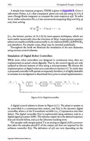
Figure 4.3.1: Digital controller.
A digital control scheme is shown in Figure 4.3.1. The plant or system to
be controlled is a continuous-time system, and K(z) is the dynamic digital
controller, where z is the Z-transform variable (i.e., z represents a unit time
-1
delay). The digital controller K(z) is implemented using software code in a
digital signal processor (DSP). The reference input r(t) is the desired trajectory
that y(t) should follow, and e k is the (discrete) tracking error.
The sampler with sample period T is an analog-to-digital (A/D) converter
that takes the samples yk=y(kT) of the output y(t) that are required by the
software controller K(z). The definition of y(t) can vary depending on the
Copyright © 2004 by Marcel Dekker, Inc.