Page 211 - Rock Mechanics For Underground Mining

FINITE DIFFERENCE METHODS FOR CONTINUOUS ROCK

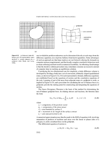
Figure 6.11 (a) Schematic finite dif- one in which the problem unknowns can be determined directly at each stage from the
ference grid; (b) representative zones difference equations, in a stepwise fashion, from known quantities. Some advantages
involved in contour integrals for a
of such an approach are that large matrices are not formed, reducing the demands on
gridpoint (after Brady and Lorig,
computer memory requirements, and that locally complex constitutive behaviour such
1988).
as strain softening need not result in numerical instability. An offsetting disadvantage
is that the iterative solution procedure may sometimes consume an excessive amount
of computer time in reaching an equilibrium solution.
Considering the two-dimensional case for simplicity, a finite difference scheme is
developed by dividing a body into a set of convenient, arbitrarily-shaped quadrilateral
zones, as shown in Figure 6.11a. For each representative domain, difference equations
are established based on the equations of motion and the constitutive equations of
the rock. Lumping of part of the mass from adjacent zones at a gridpoint or node, as
implied in Figure 6.11b, and a procedure for calculating the out-of-balance force at a
gridpoint, provide the starting point for constructing and integrating the equations of
motion.
The Gauss Divergence Theorem is the basis of the method for determining the
out-of-balance gridpoint force. In relating stresses and tractions, the theorem takes
the form
%
ij n j dS (i, j = 1, 2) (6.48)
∂ ij /∂x i = lim A→0
S
where
x i = components of the position vector
ij = components of the stress tensor
A = area bounded by surface S
dS = increment of arc length of the surface contour
n j = unit outward normal to dS.
A numerical approximation may then be made to the RHS of equation 6.48, involving
summation of products of tractions and areas over the linear or planar sides of a
polygon, to yield a resultant force on the gridpoint.
The differential equation of motion is

∂ ˚ u i /∂t = ∂ ij /∂x i + g i (6.49)
193