Page 206 - Rock Mechanics For Underground Mining

METHODS OF STRESS ANALYSIS

Introducing equation 6.41,
% % %
e T e T 0 T
[q ] = [B] [D][B][u ]dV + [B] [ ]dV − [N] [b]dV (6.42)
V e V e V e
Examining each component of the RHS of this expression, for a triangular element
& T
the term [B] [D][B]dV yields a 6 × 6 matrix of functions which must be inte-
V e
& T 0
grated over the volume of the element, the term [B] [ ]dV a6 × 1 matrix, and
V e
& T
[N] [b]dV a6 × 1 matrix. In general, the integrations may be carried out using
V e
standard quadrature theory. For a constant strain triangular element, of volume V e ,
the elements of [B] and [N] are constant over the element, and equation 6.42 becomes
e
T
0
T
T
e
[q ] = V e [B] [D][B][u ] + V e [B] [ ] − V e [N] [b]
In all cases, equation 6.42 may be written
e
e
e
e
[q ] = [K ][u ] + [f ] (6.43)
e
In this equation, equivalent internal nodal forces [q ] are related to nodal displace-
e
e
ments [u ] through the element stiffness matrix [K ] and an initial internal load vector
e
e
e
[f ]. The elements of [K ] and [f ] can be calculated directly from the element ge-
ometry, the initial state of stress and the body forces.
6.6.4 Solution for nodal displacements
The computational implementation of the finite element method involves a set of
e
e
routines which generate the stiffness matrix [K ] and initial load vector [f ] for all
elements. These data, and applied external loads and boundary conditions, provide
sufficient information to determine the nodal displacements for the complete element
assembly. The procedure is illustrated, for simplicity, by reference to the two-element
assembly shown in Figure 6.8.
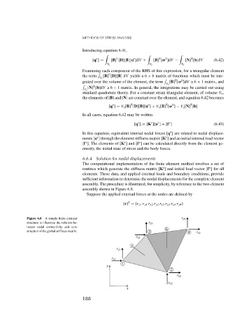
Suppose the applied external forces at the nodes are defined by
T
[r] = [r x1 r y1 r x2 r y2 r x3 r y3 r x4 r y4 ]
Figure 6.8 A simple finite element
structure to illustrate the relation be-
tween nodal connectivity and con-
struction of the global stiffness matrix.

188