Page 205 - Schaum's Outline of Differential Equations

188 NUMERICAL METHODS FOR SOLVING DIFFERENTIAL EQUATIONS [CHAP. 19

2
19.9. Use the Adams-Bashforth-Moulton method to solve / = 2xyl(x 2 - y ); (l) = 3 on the interval [1, 2]
y
with h = 0.2.
2
Here ( x , y) = 2xy/(x 2 - y ), x 0=l and y a = 3. With A = 0.2, x 1 =x a + h = 1.2, x 2 = x 1 + h = 1.4, and
f
x 3 = x 2 + h= 1.6. Using the Runge-Kutta method to obtain the corresponding y-values needed to start the
Adams-Bashforth-Moulton method, we find y 1 = 2.8232844, y 2 = 2.5709342, and y 3 = 2.1321698. It then follows
from Eq. (19.3) that

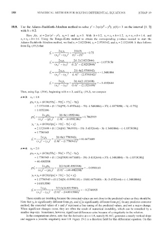
Then, using Eqs. (19.6), beginning with n = 3, and Eq. (19.3), we compute

These results are troubling because the corrected values are not close to the predicted values as they should be.
Note that y s is significantly different from py s and y' 4 is significantly different from py' 4. In any predict or-correct or
method, the corrected values of y and / represent a fine-tuning of the predicted values, and not a major change.
When significant changes occur, they are often the result of numerical instability, which can be remedied by a
smaller step-size. Sometimes, however, significant differences arise because of a singularity in the solution.
In the computations above, note that the derivative at x = 1.8, namely 81.667, generates a nearly vertical slope
and suggests a possible singularity near 1.8. Figure 19-1 is a direction field for this differential equation. On this