Page 206 - Schaum's Outline of Differential Equations

CHAP. 19] NUMERICAL METHODS FOR SOLVING DIFFERENTIAL EQUATIONS 189

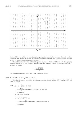
Fig. 19.1

direction field we have plotted the points (XQ, y Q) through (jc 4, y 4) as determined by the Adams-Bashforth-Moulton
method and then sketched the solution curve through these points consistent with the direction field. The cusp
between 1.6 and 1.8 is a clear indicator of a problem.
2
2
The analytic solution to the differential equation is given in Problem 4.14 as x + y = ky. Applying
the initial condition, we find k= 10/3, and then using the quadratic formula to solve explicitly for y,
we obtain the solution

This solution is only defined through x = 5/3 and is undefined after that.

19.10. Redo Problem 19.7 using Milne's method.
The values of y 0, yi, y 2, y?, and their derivatives are exactly as given in Problem 19.7. Using Eqs. (19.7) and
(19.3), we compute