Page 324 - Schaum's Outline of Theory and Problems of Advanced Calculus

CHAP. 12] IMPROPER INTEGRALS 315

The Laplace transform of a function FðxÞ is
FðxÞ lfFðxÞg
defined as
a
a 8 > 0
ð
1 sx
e FðxÞ dx 8
f ðsÞ¼ lfFðxÞg ¼ ð12Þ
0 ax 1
e 8 > a
and is analogous to power series as seen by replacing 8 a
s sx x a
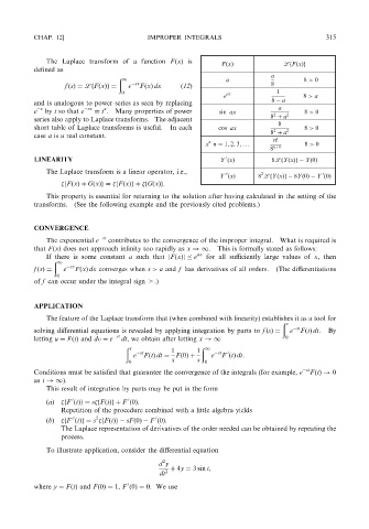
e by t so that e ¼ t . Many properties of power sin ax 2 2 8 > 0
series also apply to Laplace transforms. The adjacent 8 þ a
8
short table of Laplace transforms is useful. In each cos ax 2 2 8 > 0
case a is a real constant. 8 þ a
n!
n
x n ¼ 1; 2; 3; .. . 8 > 0
8 nþ1
LINEARITY Y ðxÞ 8lfYðxÞg Yð0Þ
0
The Laplace transform is a linear operator, i.e., 2
00 0
Y ðxÞ 8 lfYðxÞg 8Yð0Þ Y ð0Þ
fFðxÞþ GðxÞg ¼ fFðxÞg þ fGðxÞg:
This property is essential for returning to the solution after having calculated in the setting of the
transforms. (See the following example and the previously cited problems.)
CONVERGENCE
st
The exponential e contributes to the convergence of the improper integral. What is required is
that FðxÞ does not approach infinity too rapidly as x !1. This is formally stated as follows:
If there is some constant a such that jFðxÞj e ax for all sufficiently large values of x, then
ð
1
sx
e FðxÞ dx converges when s > a and f has derivatives of all orders. (The differentiations
f ðsÞ¼
0
of f can occur under the integral sign >.)
APPLICATION
The feature of the Laplace transform that (when combined with linearity) establishes it as a tool for
ð x
e st FðtÞ dt. By
solving differential equations is revealed by applying integration by parts to f ðsÞ¼
st
letting u ¼ FðtÞ and dv ¼ e dt,we obtain after letting x !1 0
x 1 1 1
ð ð
e st FðtÞ dt ¼ Fð0Þþ e st F ðtÞ dt:
0
0 s s 0
Conditions must be satisfied that guarantee the convergence of the integrals (for example, e st FðtÞ! 0
as t !1).
This result of integration by parts may be put in the form
(a) fF ðtÞg ¼ s fFðtÞg þ F ð0Þ.
0
0
Repetition of the procedure combined with a little algebra yields
2
(b) fF ðtÞg ¼ s fFðtÞg sFð0Þ F ð0Þ.
0
00
The Laplace representation of derivatives of the order needed can be obtained by repeating the
process.
To illustrate application, consider the differential equation
2
d y
þ 4y ¼ 3 sin t;
dt 2
where y ¼ FðtÞ and Fð0Þ¼ 1, F ð0Þ¼ 0. We use
0