Page 205 - Schaum's Outline of Theory and Problems of Electric Circuits

194
9.3 PHASORS SINUSOIDAL STEADY-STATE CIRCUIT ANALYSIS [CHAP. 9

A brief look at the voltage and current sinusoids in the preceding examples shows that the ampli-
tudes and phase differences are the two principal concerns. A directed line segment, or phasor, such as
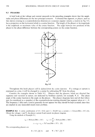
that shown rotating in a counterclockwise direction at a constant angular velocity ! (rad/s) in Fig. 9-5,
has a projection on the horizontal which is a cosine function. The length of the phasor or its magnitude
is the amplitude or maximum value of the cosine function. The angle between two positions of the
phasor is the phase difference between the corresponding points on the cosine function.

Fig. 9-5

Throughout this book phasors will be defined from the cosine function. If a voltage or current is
expressed as a sine, it will be changed to a cosine by subtracting 908 from the phase.
Consider the examples shown in Table 9-2. Observe that the phasors, which are directed line
segments and vectorial in nature, are indicated by boldface capitals, for example, V, I. The phase
angle of the cosine function is the angle on the phasor. The phasor diagrams here and all that follow
may be considered as a snapshot of the counterclockwise-rotating directed line segment taken at t ¼ 0.
The frequency f (Hz) and ! (rad/s) generally do not appear but they should be kept in mind, since they
are implicit in any sinusoidal steady-state problem.

EXAMPLE 9.3 A series combination of R ¼ 10
and L ¼ 20 mH has a current i ¼ 5:0 cos ð500t þ 108) (A).
Obtain the voltages v and V, the phasor current I and sketch the phasor diagram.
Using the methods of Example 9.1,
di
v R ¼ 50:0 cos ð500t þ 108Þ v L ¼ L ¼ 50:0 cos ð500t þ 1008Þ
dt
v ¼ v R þ v L ¼ 70:7 cos ð500t þ 558Þ ðVÞ
The corresponding phasors are

I ¼ 5:0 108 A and V ¼ 70:7 558 V