Page 103 - Schaum's Outline of Theory and Problems of Signals and Systems

LINEAR TIME-INVARIANT SYSTEMS [CHAP. 2

Thus, we can write the output y[n] as

which is sketched in Fig. 2-20(b).
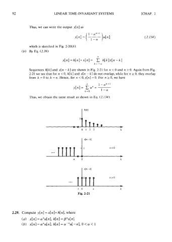
(b) By Eq. (2.39)

Sequences h[kl and x[n - k] are shown in Fig. 2-21 for n < 0 and n > 0. Again from Fig.
2-21 we see that for n < 0, h[k] and x[n - kl do not overlap, while for n 2 0, they overlap
from k = 0 to k = n. Hence, for n < 0, y[n] = 0. For n 2 0, we have

Thus, we obtain the same result as shown in Eq. (2.134).

-1 0 n
Fig. 2-21

2.29. Compute y[n] = x[n] * h[n], where

(a) x[n] = cunu[n], h[n] = pnu[n]
(b) x[n] = cunu[n], h[n] = a-"u[-n], 0 < a < 1