Page 105 - Schaum's Outline of Theory and Problems of Signals and Systems

LINEAR TIME-INVARIANT SYSTEMS [CHAP. 2

Combining Eqs. (2.136~) and (2. I36b), we obtain

(2.137)

which is sketched in Fig. 2-22.

-2-10 12 3
Fig. 2-22

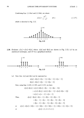
2.30. Evaluate y[n] = x[n] * h[n], where x[n] and h[n] are shown in Fig. 2-23, (a) by an
analytical technique, and (b) by a graphical method.

-10123 n -I 0 1 2 n
Fig. 2-23

(a) Note that x[n] and h[n] can be expressed as
x[n] =6[n]+6[n - l]+6[n -2]+6[n -31

h[n] = 6[n] + S[n - 1 ] + S[n - 21
Now, using Eqs. (2.38), (2.130), and (2. I3l), we have
x[n] * h[n] = x[n] * {S[n] + 6[n - 1 ] + 6[n - 21)
*
= ~[n] S[n] +x[n] * S[n - I ] + x[n] * S[n - 21)
=x[n] +x[n - 1] +x[n - 21
Thus, y[n] = S[n] + S[n - I] + S[n - 21 + 6[n - 31

+6[n- 1]+8[n-2]+6[n-3]+6[n-41
+S[n-2]+6[n-3]+6[n-4]+6[n-5]
or y[n] = S[n] + 2S[n - 1] + 36[n - 21 + 36[n - 31 + 26[n - 41 + 6[n - 51

or Y[~I= {1,2,3,3,2,l}