Page 80 - Schaum's Outline of Theory and Problems of Signals and Systems

CHAP. 21 LINEAR TIME-INVARIANT SYSTEMS

(b) By Eq. (2.10)

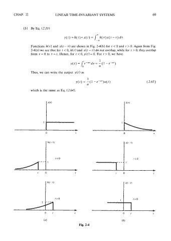
Functions h(r) and x(t - 7) are shown in Fig. 2-4(b) for t < 0 and t > 0. Again from Fig.
2-4(b) we see that for t < 0, h(7) and x(t - 7) do not overlap, while for t > 0, they overlap
from 7 = 0 to r = t. Hence, for t < 0, y(t) = 0. For t > 0, we have

Thus, we can write the output y(t) as

which is the same as Eq. (2.64).

(a)
Fig. 2-4