Page 79 - Schaum's Outline of Theory and Problems of Signals and Systems

LINEAR TIME-INVARIANT SYSTEMS [CHAP. 2

(dl In a similar manner, we have

m
x(t) * u(t - t,,) = x(r)u(t - 7 -to) dr =

2.3. Let y(r) = x(r) * h(t 1. Then show that

By Eq. (2.6) we have

and

Let r - t, = A. Then T = A + t, and Eq. (2.63b) becomes

Comparing Eqs. (2.63~) and (2.63~1, we see that replacing I in Eq. (2.63~) by r - r , - r,, we
obtain Eq. (2.63~). Thus, we conclude that

2.4. The input x(t) and the impulse response h(t) of a continuous time LTI system are
given by

(a) Compute the output y(t) by Eq. (2.6).
(b) Compute the output y(t) by Eq. (2.10).
(a) By Eq. (2.6)

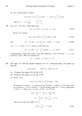
Functions X(T) and h(t - r) are shown in Fig. 2-4(a) for t < 0 and t > 0. From Fig. 2-4(a)
we see that for t < 0, x(r) and h(t - T) do not overlap, while for t > 0, they overlap from
T = 0 to T = I. Hence, for t < 0, y(t) = 0. For t > 0, we have

Thus, we can write the output y(t) as