
Page 83 - Schaum's Outline of Theory and Problems of Signals and Systems
P. 83
LINEAR TIME-INVARIANT SYSTEMS [CHAP. 2
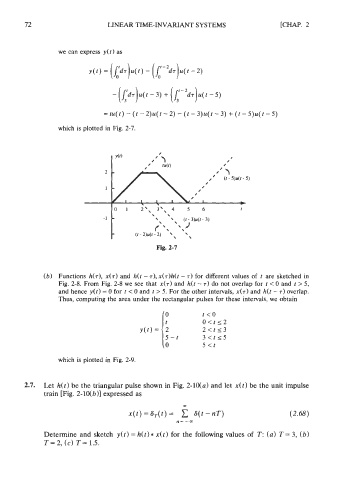
we can express y(t ) as
= tu(t) - (t - 2)u(t - 2) - (t - 3)u(t - 3) + (r - 5)u(t - 5)
which is plotted in Fig. 2-7.
Fig. 2-7
(b) Functions h(r), X(T) and h(t - 71, x(r)h(t - 7) for different values of t are sketched in
Fig. 2-8. From Fig. 2-8 we see that x(r) and h(t - 7) do not overlap for t < 0 and t > 5,
and hence y(t) = 0 for t < 0 and t > 5. For the other intervals, x(r) and h(t - T) overlap.
Thus, computing the area under the rectangular pulses for these intervals, we obtain
which is plotted in Fig. 2-9.
2.7. Let h(t) be the triangular pulse shown in Fig. 2-10(a) and let x(t) be the unit impulse
train [Fig. 2-10(b)] expressed as
Determine and sketch y(t) = h(t) * x( t) for the following values of T: (a) T = 3, (b)
T = 2, (c) T = 1.5.