Page 82 - Schaum's Outline of Theory and Problems of Signals and Systems
P. 82

CHAP.  21                 LINEAR TIME-INVARIANT SYSTEMS


                  Combining Eqs. (2.66~) and (2.6681, we can write y(t) as
                                                       1
                                               y(t) = -e-uIrl      CY>O
                                                      2a

                  which is shown in  Fig. 2-Sb).


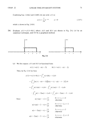
            2.6.   Evaluate  y(t) =x(t) * h(t ),  where  x(t) and  h(t) are  shown  in  Fig.  2-6,  (a) by  an
                  analytical  technique, and (b) by a graphical method.


                                0    1   2    3   1
                                                     Fig. 2-6


                  (a)  We first express  x(t  and h(t) in functional form:


                       Then, by Eq. (2.6) we  have


                                                                     O<r<t,t>O
                       Since                 u(7)u(t - 7) =
                                                                     otherwise

                                         u(r)u(t - 2 - 7) =  (A      0<7<t-2,t>2
                                                                     otherwise

                                                                     3<7<t,t>3
                                         ~(7- 3)u(t - 7) =
                                                                     otherwise
                                                                     3<~<t-2,t>5
                                      U(T-~)U(~-~-T)
                                                         =
                                                                    otherwise
   77   78   79   80   81   82   83   84   85   86   87