Page 90 - Schaum's Outline of Theory and Problems of Signals and Systems

CHAP. 21 LINEAR TIME-INVARIANT SYSTEMS

Using Eqs. (2.61) and (2.9), Eq. (2.73) can be expressed as

Thus, we obtain
-T/2<tr T/2 ( 2.75)
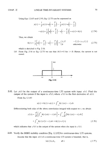
h(t) = :[~(t+
T
f) -u(~- f)] 0 otherwise
=
which is sketched in Fig. 2-16.
(b) From Fig. 2-16 or Eq. (2.75) we see that h(t) # 0 for t < 0. Hence, the system is not
causal.

-Tn 0 rn t
Fig. 2-16

2.12. Let y(t) be the output of a continuous-time LTI system with input x(t). Find the
output of the system if the input is xl(t), where xl(t) is the first derivative of x(t).
From Eq. (2.10)

Differentiating both sides of the above convolution integral with respect to 1, we obtain

which indicates that yl(t) is the output of the system when the input is xl(t).

2.13. Verify the BIB0 stability condition [Eq. (2.21)] for continuous-time LTI systems.
Assume that the input x(t) of a continuous-time LTI system is bounded, that is,

Ix(t)ll k, all t (2.77)