Page 94 - Schaum's Outline of Theory and Problems of Signals and Systems

CHAP. 21 LINEAR TIME-INVARIANT SYSTEMS 83

Since cos wr is an even function of w, changing w to -w in Eq. (2.90) and changing j to -j in
Eq. (2.891, we have
m
H( -jw) = H( jw)* = 2/ h(r) COS( -or) dr
0
= 2jrnh(r) cos or dr = H( jw)
0
Thus, we see that the eigenvalue H(jw) corresponding to the eigenfunction el"' is real. Let the
system be represented by T. Then by Eqs. (2.231, (2.241, and (2.91) we have

T(ejU'} = H( jw) e'"' (2.92~)
T[~-J"'} H( -jw) e-J"' = H( jo) e-I"' ( 2.92b)
=
Now, since T is linear, we get
T[COS ot} = T{;(ej"' + e-'"I )} = ;T(~J~'} + :T(~-J"' 1

+
= ~(j~){;(~j"' )} = ~(jw)cos wt (2.93~)
e-Jwr

Thus, from Eqs. (2.93~) and (2.93b) we see that cos wt and sin wt are the eigenfunctions of the
system with the same real eigenvalue H( jo) given by Eq. (2.88) or (2.90).

SYSTEMS DESCRIBED BY DIFFERENTIAL EQUATIONS

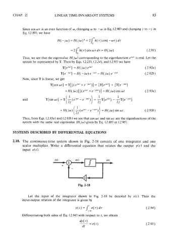
2.18. The continuous-time system shown in Fig. 2-18 consists of one integrator and one
scalar multiplier. Write a differential equation that relates the output y( t ) and the
input x( t 1.

Fig. 2-18

Let the input of the integrator shown in Fig. 2-18 be denoted by e(t). Then the
input-output relation of the integrator is given by

Differentiating both sides of Eq. (2.94) with respect to t, we obtain