Page 92 - Schaum's Outline of Theory and Problems of Signals and Systems

CHAP . 21 LINEAR TIME-INVARIANT SYSTEMS

(6) Using the above h( t ), we have

=2(1-+)=I <a:

Thus, the system is BIB0 stable.

EIGENFUNCTIONS OF CONTINUOUS-TIME LTI SYSTEMS

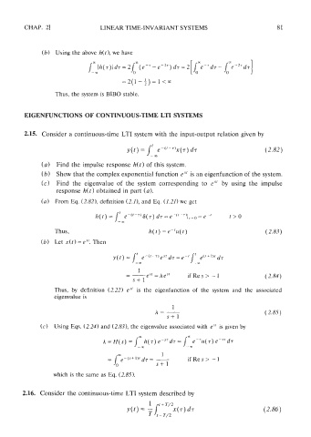
2.15. Consider a continuous-time LTI system with the input-output relation given by

y(t) = 1' e-('-''x(r) dr (2.82)
-03
(a) Find the impulse response h(t) of this system.
(b) Show that the complex exponential function e"' is an eigenfunction of the system.
(c) Find the eigenvalue of the system corresponding to eS' by using the impulse
response h(t) obtained in part (a).
(a) From Eq. (2.821, definition (2.1), and Eq. (1.21) we get

h(f ) = /' e-(1-T)6(7) d7 = e-('-')I7= 0-e t > O
-
- m
Thus, h(t) = e-'~(1) ( 2.83)
(6) Let x(f ) = e". Then

Thus, by definition (2.22) e" is the eigenfunction of the system and the associated
eigenvalue is

(c) Using Eqs. (2.24) and (2.83), the eigenvalue associated with e"' is given by

which is the same as Eq. (2.85).

2.16. Consider the continuous-time LTI system described by