Page 180 - Schaum's Outlines - Probability, Random Variables And Random Processes

CHAP. 51 RANDOM PROCESSES 173

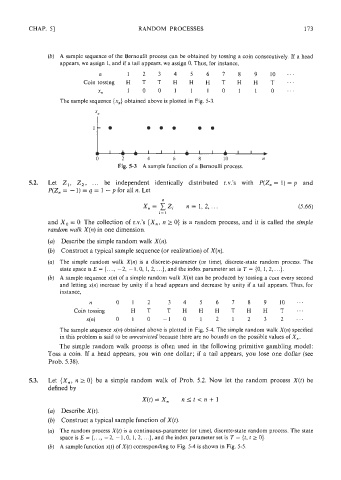
(b) A sample sequence of the Bernoulli process can be obtained by tossing a coin consecutively. If a head
appears, we assign 1, and if a tail appears, we assign 0. Thus, for instance,
n 1 2 3 4 5 6 7 8 9 1 0 . - .
Coin tossing H T T H H H T H H T . . .
xn 1 0 0 1 1 1 0 1 1 0 ~ ~ ~
The sample sequence {x,} obtained above is plotted in Fig. 5-3.

I- 0 0 . . 0 .

-
I A I I A I I )
0 2 4 6 8 10 n
Fig. 5-3 A sample function of a Bernoulli process.

5.2. Let Z,, Z,, . . . be independent identically distributed r.v.'s with P(Zn = 1) = p and
P(Z, = - 1) = q = 1 - p for all n. Let

and X, = 0. The collection of r.v.'s {X,, n > 0) is a random process, and it is called the simple
random walk X(n) in one dimension.

(a) Describe the simple random walk X(n).
(b) Construct a typical sample sequence (or realization) of X(n).

(a) The simple random walk X(n) is a discrete-parameter (or time), discrete-state random process. The
state space is E = (. . . , -2, - 1,0, 1, 2,. . .), and the index parameter set is T = (0, 1,2, . . .).
(b) A sample sequence x(n) of a simple random walk X(n) can be produced by tossing a coin every second
and letting x(n) increase by unity if a head appears and decrease by unity if a tail appears. Thus, for
instance,
n 0 1 2 3 4 5 6 7 8 9 10
Coin tossing H T T H H H T H H T - m e
x(n) 0 1 0 - 1 0 1 2 1 2 3 2 - a .
The sample sequence x(n) obtained above is plotted in Fig. 5-4. The simple random walk X(n) specified
in this problem is said to be unrestricted because there are no bounds on the possible values of X, .
The simple random walk process is often used in the following primitive gambling model:
Toss a coin. If a head appears, you win one dollar; if a tail appears, you lose one dollar (see
Prob. 5.38).

5.3. Let (x,, n 2 0) be a simple random walk of Prob. 5.2. Now let the random process X(t) be
defined by
X(t)=Xn n<t<n+l
(a) Describe X(t).
(b) Construct a typical sample function of X(t).
(a) The random process X(t) is a continuous-parameter (or time), discrete-state random process. The state
space is E = {. . . , -2, - 1,0, 1,2,. . .}, and the index parameter set is T = (t, t 2 0).
(b) A sample function x(t) of X(t) corresponding to Fig. 5-4 is shown in Fig. 5-5.