Page 181 - Schaum's Outlines - Probability, Random Variables And Random Processes

RANDOM PROCESSES [CHAP 5

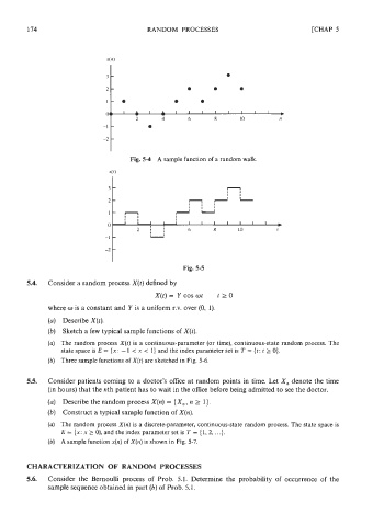
Fig. 5-4 A sample function of a random walk.

Fig. 5-5

Consider a random process X(t) defined by
X(t) = Y cos ot t 2 0
where o is a constant and Y is a uniform r.v. over (0, 1).
(a) Describe X(t).
(b) Sketch a few typical sample functions of X(t).
(a) The random process X(t) is a continuous-parameter (or time), continuous-state random process. The
state space is E = {x: - 1 < x < 1) and the index parameter set is T = {t: t 2 0).
(b) Three sample functions of X(t) are sketched in Fig. 5-6.

Consider patients coming to a doctor's office at random points in time. Let X, denote the time
(in hours) that the nth patient has to wait in the office before being admitted to see the doctor.
(a) Describe the random process X(n) = {X,, n 2 1).
(b) Construct a typical sample function of X(n).
(a) The random process X(n) is a discrete-parameter, continuous-state random process. The state space is
E = {x: x 2 0)' and the index parameter set is T = (1'2, . . .).
(b) A sample function x(n) of X(n) is shown in Fig. 5-7.

CHARACTERIZATION OF RANDOM PROCESSES
5.6. Consider the Bernoulli process of Prob. 5.1. Determine the probability of occurrence of the
sample sequence obtained in part (b) of Prob. 5.1.