Page 55 - Probability, Random Variables and Random Processes

CHAP. 21 RANDOM VARIABLES 47

F. Normal (or Gaussian) Distribution:
A r.v. X is called a normal (or gaussian) r.v. if its pdf is given by

The corresponding cdf of X is

This integral cannot be evaluated in a closed form and must be evaluated numerically. It is conve-
nient to use the function @(z), defined as

to help us to evaluate the value of FX(x). Then Eq. (2.53) can be written as

Note that

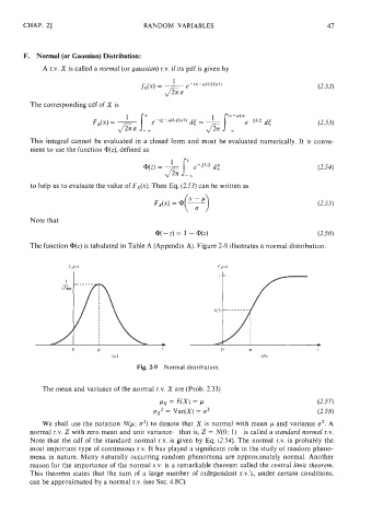
The function @(z) is tabulated in Table A (Appendix A). Figure 2-9 illustrates a normal distribution.

Fig. 2-9 Normal distribution.

The mean and variance of the normal r.v. X are (Prob. 2.33)

We shall use the notation N(p; a2) to denote that X is normal with mean p and variance a2. A
normal r.v. Z with zero mean and unit variance-that is, Z = N(0; 1)-is called a standard normal r.v.
Note that the cdf of the standard normal r.v. is given by Eq. (2.54). The normal r.v. is probably the
most important type of continuous r.v. It has played a significant role in the study of random pheno-
mena in nature. Many naturally occurring random phenomena are approximately normal. Another
reason for the importance of the normal r.v. is a remarkable theorem called the central limit theorem.
This theorem states that the sum of a large number of independent r.v.'s, under certain conditions,
can be approximated by a normal r.v. (see Sec. 4.8C).