Page 170 - Sensing, Intelligence, Motion : How Robots and Humans Move in an Unstructured World

MAXIMUM TURN STRATEGY 145

other; if they do, they are considered one obstacle. The total number of obstacles
in the scene need not be finite.
The robot’s sensors provide it with information about its surroundings within
the sensing range (radius of vision), a disc of radius r v centered at its current
location C i . The sensor can assess the distance to the nearest obstacle in any
direction within the sensing range. The robot input information at moment t i
includes its current velocity vector V i , coordinates of point C i and of the target
point T , and possibly few other points of interest that will be discussed later.
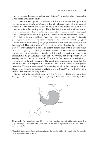
The task is to move, collision-free, from point S (start) to point T (target)
(see Figure 4.1). The robot’s control means include two components (p, q)of
f
the acceleration vector u = = (p, q),where m is the robot mass and f is the
m
force applied. Though the units of (p, q) are those of acceleration, by normalizing
to m = 1 we can refer to p and q as control forces, each within its fixed range
|p|≤ p max , |q|≤ q max .Force p controls forward (or backward when braking)
motion; its positive direction coincides with the velocity vector V.Force q is
perpendicular to p, forming a right pair of vectors, and is equivalent to the
steering control (rotation of vector V) (Figure 4.2). Constraints on p and q imply
a constraint on the path curvature. The point mass assumption implies that the
robot’s rotation with respect to its “center of mass” has no effect on the system
dynamics. There are no external forces acting on the robot except p and q.
There is no friction; for example, values p = q = 0and V = 0 will result in a
straight-line constant velocity motion. 2
Robot motion is controlled in steps i, i = 0, 1, 2,... . Each step takes time
δt = t i+1 − t i = const. The step’s length depends on the robot’s velocity within

Robot’s path
T
Q

P L

C
Obstacle
H

S M-line
r u

Figure 4.1 An example of a conflict between the performance of a kinematic algorithm
(e.g., VisBug-21, the solid line path) and the effects of dynamics (the dotted piece of
trajectory at P).

2 If needed, other external forces and constraints can be handled within this model, using for example
the technique described in Ref. 95.