Page 326 - Sensing, Intelligence, Motion : How Robots and Humans Move in an Unstructured World

THE CASE OF THE PPP (CARTESIAN) ARM 301

V-plane and the Type III obstacle in the only possible local direction, as
in Motion III.
3. Another Type III obstacle is encountered. Then there will be a nonzero
projection of the intersection curve between two Type III obstacles onto
C p ;the P c (C-point) will continue following the obstacle boundary. Accord-
ingly, the C-point will follow the intersection curve between the two Type
III obstacles in the only possible local direction, see Motion V.
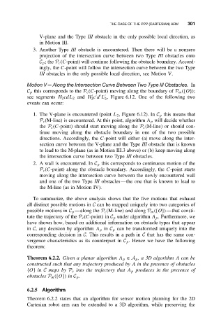
Motion V—Along the Intersection Curve Between Two Type III Obstacles. In
C p this corresponds to the P c (C-point) moving along the boundary of P m ({O});

see segments H 2 cdL 2 and H c d L , Figure 6.12. One of the following two

2 2
events can occur:
1. The V-plane is encountered (point L 2 , Figure 6.12). In C p this means that
P c (M-line) is encountered. At this point, algorithm A p will decide whether
the P c (C-point) should start moving along the P c (M-line) or should con-
tinue moving along the obstacle boundary in one of the two possible
directions. Accordingly, the C-point will either (a) move along the inter-
section curve between the V-plane and the Type III obstacle that is known
to lead to the M-plane (as in Motion III.3 above) or (b) keep moving along
the intersection curve between two Type III obstacles.
2. A wall is encountered. In C p this corresponds to continuous motion of the
P c (C-point) along the obstacle boundary. Accordingly, the C-point starts
moving along the intersection curve between the newly encountered wall
and one of the two Type III obstacles—the one that is known to lead to
the M-line (as in Motion IV).

To summarize, the above analysis shows that the five motions that exhaust
all distinct possible motions in C can be mapped uniquely into two categories of
possible motions in C p —along the P c (M-line) and along P m ({O})—that consti-
tute the trajectory of the P c (C-point) in C p under algorithm A p .Furthermore,we
have shown how, based on additional information on obstacle types that appear
in C, any decision by algorithm A p in C p can be transformed uniquely into the
corresponding decision in C. This results in a path in C that has the same con-
vergence characteristics as its counterpart in C p . Hence we have the following
theorem:
Theorem 6.2.2. Given a planar algorithm A p ∈ A p , a 3D algorithm A can be
constructed such that any trajectory produced by A in the presence of obstacles
{O} in C maps by P c into the trajectory that A p produces in the presence of
obstacles P m ({O}) in C p .

6.2.5 Algorithm

Theorem 6.2.2 states that an algorithm for sensor motion planning for the 2D
Cartesian robot arm can be extended to a 3D algorithm, while preserving the