Page 330 - Sensing, Intelligence, Motion : How Robots and Humans Move in an Unstructured World

THREE-LINK XXP ARM MANIPULATORS 305

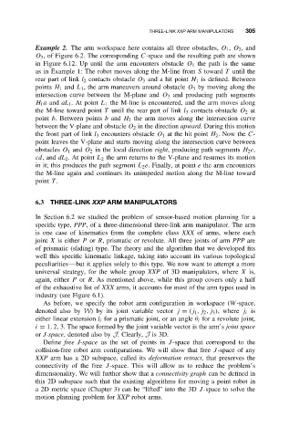
Example 2. The arm workspace here contains all three obstacles, O 1 , O 2 ,and
O 3 , of Figure 6.2. The corresponding C-space and the resulting path are shown
in Figure 6.12. Up until the arm encounters obstacle O 1 the path is the same
as in Example 1: The robot moves along the M-line from S toward T until the
rear part of link l 2 contacts obstacle O 3 and a hit point H 1 is defined. Between
points H 1 and L 1 , the arm maneuvers around obstacle O 3 by moving along the
intersection curve between the M-plane and O 3 and producing path segments
H 1 a and aL 1 . At point L 1 the M-line is encountered, and the arm moves along
the M-line toward point T until the rear part of link l 3 contacts obstacle O 2 at
point b. Between points b and H 2 the arm moves along the intersection curve
between the V-plane and obstacle O 2 in the direction upward. During this motion
the front part of link l 3 encounters obstacle O 1 at the hit point H 2 .Now the C-
point leaves the V-plane and starts moving along the intersection curve between
obstacles O 1 and O 2 in the local direction right, producing path segments H 2 c,
cd,and dL 2 . At point L 2 the arm returns to the V-plane and resumes its motion
in it; this produces the path segment L 2 e. Finally, at point e the arm encounters
the M-line again and continues its unimpeded motion along the M-line toward
point T .

6.3 THREE-LINK XXP ARM MANIPULATORS

In Section 6.2 we studied the problem of sensor-based motion planning for a
specific type, PPP, of a three-dimensional three-link arm manipulator. The arm
is one case of kinematics from the complete class XXX of arms, where each
joint X is either P or R, prismatic or revolute. All three joints of arm PPP are
of prismatic (sliding) type. The theory and the algorithm that we developed fits
well this specific kinematic linkage, taking into account its various topological
peculiarities—but it applies solely to this type. We now want to attempt a more
universal strategy, for the whole group XXP of 3D manipulators, where X is,
again, either P or R. As mentioned above, while this group covers only a half
of the exhaustive list of XXX arms, it accounts for most of the arm types used in
industry (see Figure 6.1).
As before, we specify the robot arm configuration in workspace (W-space,
denoted also by W) by its joint variable vector j = (j 1 ,j 2 ,j 3 ),where j i is
either linear extension l i for a prismatic joint, or an angle θ i for a revolute joint,
i = 1, 2, 3. The space formed by the joint variable vector is the arm’s joint space
or J-space, denoted also by J. Clearly, J is 3D.
Define free J-space as the set of points in J-space that correspond to the
collision-free robot arm configurations. We will show that free J-space of any
XXP arm has a 2D subspace, called its deformation retract, that preserves the
connectivity of the free J-space. This will allow us to reduce the problem’s
dimensionality. We will further show that a connectivity graph canbedefinedin
this 2D subspace such that the existing algorithms for moving a point robot in
a 2D metric space (Chapter 3) can be “lifted” into the 3D J-space to solve the
motion planning problem for XXP robot arms.