Page 169 - Separation process engineering

One known point is the intercept of the top operating line with the feed line. We still need a second
point, and we can find it at the x intercept. When y is set to zero, x = x (this is left as Problem 4.C1).
B
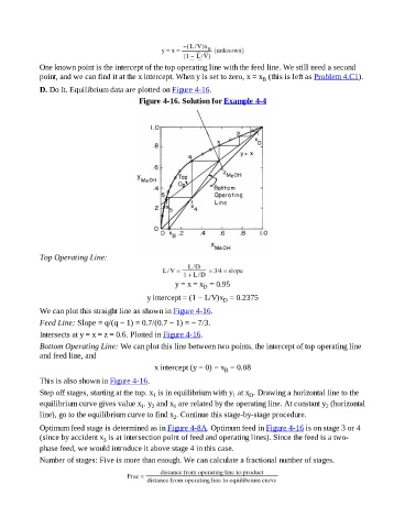
D. Do It. Equilibrium data are plotted on Figure 4-16.

Figure 4-16. Solution for Example 4-4

Top Operating Line:

y = x = x = 0.95
D
y intercept = (1 − L/V)x = 0.2375
D
We can plot this straight line as shown in Figure 4-16.

Feed Line: Slope = q/(q − 1) = 0.7/(0.7 − 1) = − 7/3.

Intersects at y = x = z = 0.6. Plotted in Figure 4-16.
Bottom Operating Line: We can plot this line between two points, the intercept of top operating line
and feed line, and

x intercept (y = 0) = x = 0.08
B
This is also shown in Figure 4-16.
Step off stages, starting at the top. x is in equilibrium with y at x . Drawing a horizontal line to the
1
1
D
equilibrium curve gives value x . y and x are related by the operating line. At constant y (horizontal
1
1
2
2
line), go to the equilibrium curve to find x . Continue this stage-by-stage procedure.
2
Optimum feed stage is determined as in Figure 4-8A. Optimum feed in Figure 4-16 is on stage 3 or 4
(since by accident x is at intersection point of feed and operating lines). Since the feed is a two-
3
phase feed, we would introduce it above stage 4 in this case.
Number of stages: Five is more than enough. We can calculate a fractional number of stages.