Page 88 - Separation process principles 2

2.6 Activity-Coefficient Models for the Liquid Phase 53

coefficients at infinite dilution. Applying (3) of Table 2.9 to (1)ln-hexane (2), a system of this type, at 101.3 kPa. These
the conditions xi = 0 and then x, = 0, we have data were correlated with the van Laar equation by Orye
and Prausnitz [36] to give A12 = 2.409 and = 1.970.
From xl = 0.1 to 0.9, the fit of the data to the van Laar
and equation is reasonably good; in the dilute regions, however,
Aji = lnyjm, xj = 0 (2-72) deviations are quite severe and the predicted activity coeffi-
cients for ethanol are low. An even more serious problem
For practical applications, it is important that the van Lax with these highly nonideal mixtures is that the van Laar
equation predicts azeotrope formation correctly, where equation may erroneously predict formation of two liquid
xi = yi and Ki = 1 .O. If activity coefficients are known or can phases (phase splitting) when values of activity coefficients
be computed at the azeotropic composition-say, from exceed approximately 7.
(2-69), (yiL = P/ PiS, since Ki = 1.0)-these coefficients
can be used to determine the van Laar constants directly
Local-Composition Concept and the Wilson Model
from the following equations obtained by solving simultane-
ously for A12 and A211 Since its introduction in 1964, the Wilson equation [37],
( :; :: : shown in binary form in Table 2.9 as (4), has received wide
2
)
attention because of its ability to fit strongly nonideal, but
A12 = lnyl 1 + - (2-73) miscible, systems. As shown in Figure 2.16, the Wilson equa-
( tion, with binary interaction parameters of A12 = 0.0952 and
A21=lny2 I+- lnyl)' (2-74) 1\21 = 0.2713 determined by Orye and Prausnitz [36], fits
X2 In 72
experimental data well even in dilute regions where the vari-
These equations are applicable to activity-coefficient data ation of yl becomes exponential. Corresponding infinite-
obtained at any single composition. dilution activity coefficients computed from the Wilson
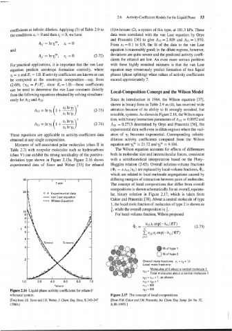
Mixtures of self-associated polar molecules (class I1 in equation are y? = 21.72 and y? = 9.104.
Table 2.7) with nonpolar molecules such as hydrocarbons The Wilson equation accounts for effects of differences
(class V) can exhibit the strong nonideality of the positive- both in molecular size and intermolecular forces, consistent
deviation type shown in Figure 2.15a. Figure 2.16 shows with a semitheoretical interpretation based on the Flory-
experimental data of Sinor and Weber [35] for ethanol Huggins relation (2-65). Overall solution-volume fractions
(Qi = xi viL/vL) are replaced by local-volume fractions, &i,
which are related to local-molecule segregations caused by
30 differing energies of interaction between pairs of molecules.
The concept of local compositions that differ from overall
compositions is shown schematically for an overall, equimo-
20
0 A Experimental data lar, binary solution in Figure 2.17, which is taken from
- van Laar equation
Wilson Equation Cukor and Prausnitz [38]. About a central molecule of type
1, the local mole fraction of molecules of type 2 is shown as
i, while the overall composition is i.
10
9 For local-volume fraction, Wilson proposed
8
7
6 = Vi~xi exp(-Aii/RT)
6 (2-75)
Y C
5 vj~x, exp(-Aij/RT)
j=1
4
3
@ 15 of type 1
0 type 2
of
15
2
Overall mole fractions: x, = x2 = '12
Local mole fractions:
Molecules of 2 about a central molecule 1
"' = Total molecules about a central molecule 1
=
xz1 + x,~ 1, as shown
1 .O 2.0 4.0 6.0 8.0 1:0 x12+xz2= 1
Xethanol 11 1 - 318
Figure 2.16 Liquid-phase activity coefficients for ethanol/ x2, - 518
n-hexane system. Figure 2.17 The concept of local compositions.
[Data from J.E. Sinor and J.H. Weber, J. Chem. Eng. Data, 5,243-247 [From P.M. Cukor and J.M. Prausnitz, Int. Chem. Eng. Symp. Ser. No. 32,
(1960).] 3,88 (1969).]