Page 84 - Separation process principles 2

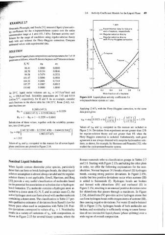
2.6 Activity-Coefficient Models for the Liquid Phase 49

EXAMPLE 2.7
I atm
yerazunis, plowright, and Smola [31] measured liquid-phase activ-
- aO Experimental data for toluene -
ity coefficients for the n-heptaneltoluene system over the entire and n-heptane, respectively
concentration range at 1 atm (101.3 kPa). Estimate activity coef- - Regular solution theory
ficients for the range of conditions using regular-solution theory Regular solution theory
both with and without the Flory-Huggins correction. Compare with Flory-Huggins correction -
values with experimental data.

-
SOLUTION
Experimental liquid-phase compositions and temperatures for 7 of 19
points are as follows, where H denotes heptane andT denotes toluene:
T, "c XH XT
98.41 1 .OOOO 0.0000
98.70 0.9154 0.0846
99.58 0.7479 0.2521
101.47 0.5096 0.4904 1.1 - -
104.52 0.2681 0.7319
107.57 0.1087 0.8913
110.60 0.0000 1 .OOOO
0 0.2 0.4 0.6 0.8 1 .O
~t 25"C, liquid molar volumes are VH, = 147.5 cm3/mol and Mole fraction of n-heptane
e, 106.8 cm3/n~ol. Solubility parameten are 7.43 and 8.914
=
Figure Z.L4 Liquid-phase activity coefficients for
(ca~cm')"~, respectively, for H and T. As an example, consider n-heptaneltoluene system at atm.
mole fractions in the above table for 104.52"C. From (2-62), vol-
ume fractions are
0.2681(147.5) Applying (2-67), with the Flory-Huggins correction, to the same
QH = = 0.3359 data point gives
0.2681(147.5) + 0.7319(106.8)
QT = 1 - QH = 1 - 0.3359 = 0.6641 [ ( 147.5) + ( 147.5 )]
1
y~=exp 0.1923+ln - - - 1.179
=
Substitution of these values, together with the solubility parame- 117.73 117.73
ters, into (2-64) gives
Values of y H and y~ computed in this manner are included in
147.5[7.430 - 0.3359(7.430) - 0.6641(8.914)12 Figure 2.14. Deviations from experiment are not greater than 12%
Y~=exp
1.987(377.67) for regular-solution theory and not greater than 6% when the
Flory-Huggins correction is included. Unfortunately, such good
= 1.212
agreement is not always obtained with nonpolar hydrocarbon solu-
Values of y~ and y~ computed in this manner for all seven liquid- tions, as shown, for example, by Hermsen and Prausnitz [32], who
phase conditions are plotted in Figure 2.14. studied the cyclopentane/benzene system.

Roman numerals refer to classification groups in Tables 2.7
Nonideal Liquid Solutions
and 2.8. Starting with Figure 2.15a and taking the other plots
When liquids contain dissimilar polar species, particularly in order, we offer the following explanations for the non-
those that can form or break hydrogen bonds, the ideal-liquid idealities. Normal heptane (V) breaks ethanol (11) hydrogen
solution assumption is almost always invalid and the regular- bonds, causing strong positive deviations. In Figure 2.15b,
solution theory is not applicable. Ewell, Harrison, and Berg similar but less positive deviations occur when acetone (111)
[33] provide a very useful classification of molecules based is added to formamide (I). Hydrogen bonds are broken
on the potential for association or solvation due to hydrogen- and formed with chloroform (IV) and methanol (11) in
bond formation. If a molecule contains a hydrogen atom at- Figure 2.15c, resulting in an unusual positive deviation curve
tached to a donor atom (0, N, F, and in certain cases C), the for chloroform that passes through a maximum. In Figure
active hydrogen atom can form a bond with another molecule 2.15d, chloroform (IV) provides active hydrogen atoms that
containing a donor atom. The classification in Table 2.7 per- can form hydrogen bonds with oxygen atoms of acetone (111),
mits qualitative estimates of deviations from Raoult's law for thus causing negative deviations. For water (I) and n-butanol
binary pairs when used in conjunction with Table 2.8. Posi- (11) in Figure 2.15e, hydrogen bonds of both molecules are
tive deviations correspond to values of yiL > 1. Nonideality broken, and nonideality is sufficiently strong to cause forma-
results in a variety of variations of y,~ with composition, as tion of two immiscible liquid phases (phase splitting) over a
shown in Figure 2.15 for several binary systems, where the wide region of overall composition.