Page 243 -

11 How Many Times Should One Run a Computational Simulation? 241

passing and postponement. In that source, the authors state that, based on 100 runs,
the average number of decisions by resolution (resp., by oversight) is 43:90 (resp.,
779:57) under anarchy (group 1), 24:82 (resp., 461:94) under competent hierarchy
(group 2) and 7:71 (resp., 192:77) under incompetent hierarchy (group 3). We can
approximate the average value of the ratio r ro through the ratio of the averages, i.e.
N x 1 ' 0:0563, Nx 2 ' 0:0537 and Nx 3 ' 0:0400. Therefore, we expect the difference
between the average value of r ro in competent hierarchy with respect to anarchy to
be around Nx 2 Nx 1 ' 0:0026, and in incompetent hierarchy with respect to anarchy
to be around Nx 3 Nx 1 ' 0:016. These coefficients are remarkably near to the ones
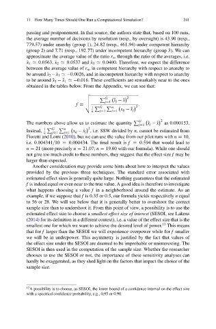
obtained in the tables below. From the Appendix, we can see that:

v
P G 2
u
jD1
u N x j Nx
t :
f D 2
1 P G P n
n jD1 iD1 x ij Nx j
G 2
P
The numbers above allow us to estimate the quantity N x j Nx as 0:000153.
jD1
2

Instead, 1 P G P n x ij Nx j , i.e. SSW divided by n, cannot be estimated from
n jD1 iD1
Fioretti and Lomi (2010), but we can use the value from our pilot runs with n D 10,
i.e. 0:004341=10 D 0:000434. The final result is f D 0:594 that would lead to
n D 21 (more precisely n D 21:07; n D 19:60 with our formula). While one should
not give too much credit to these numbers, they suggest that the effect size f may be
larger than expected.
Another consideration may provide some hints about how to interpret the values
provided by the previous three techniques. The standard error associated with
estimated effect sizes is generally quite large. Nothing guarantees that the estimated
f is indeed equal or even near to the true value. A good idea is therefore to investigate
what happens choosing a value f in a neighborhood around the estimate. As an
example, if we suppose that f is 0:35 or 0:5, our formula yields respectively n equal
to 56 or 28. We will see below that it is generally better to overshoot the correct
sample size than to undershoot it. From this point of view, a possibility is to use the
estimated effect size to choose a smallest effect size of interest (SESOI, see Lakens
(2014) for its definition in a different context), i.e. a value of the effect size that is the
13
smallest one for which we want to achieve the desired level of power. This means
that for f larger than the SESOI we will experience overpower while for f smaller
we will be in underpower. This asymmetry is justified by the fact that values of
the effect size under the SESOI are deemed to be improbable or uninteresting. The
SESOI is then used in the computation of the sample size. Whether the researcher
chooses to use the SESOI or not, the importance of these sensitivity analyses can
hardly be exaggerated, as they shed light on the factors that impact the choice of the
sample size.

13
A possibility is to choose, as SESOI, the lower bound of a confidence interval on the effect size
with a specified confidence probability, e.g., 0.95 or 0.90.