Page 246 -

244 R. Seri and D. Secchi

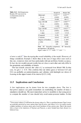
Table 11.3 OLS Regression Model 40 Model 500
Results (DV: decisions by
resolution/decisions by (Intercept) 0:056 0:055
oversight) St. err. (0.002) (0.001)
t value 29.804 100.12
Type: HC/AR 0:007 0:005
St. err. (0.003) (0.001)
t value 2:692 5:99
Type: HI/AR 0:012 0:015
St. err. (0.003) (0.001)
t value 4:637 19:18
R-squared 0.156 0.205
F-statistic 10.842 192.497
Degrees of freedom 2, 117 2, 1497
p-value 0.000 0.000
N 120 1500
Note. HC hierarchy-competence, HI hierarchy-
incompetence, AR anarchy
Signif. codes: 0 “***” 0.001 “**” 0.01 “ ” 1

15
of error ˛ and ˇ, thus decreasing the overall reliability of the model. However, all
things considered, Example 2 shows that, in the case of large effect sizes such as
this one, overpower does not bear particularly relevant problems besides accuracy.
In fact, the two models present results that are close to each other and only differ in
the granularity and reliability of details.
One last remark concerns the value of f as estimated from Model 500. In that
case, we get f D 0:51. This confirms that our initial guess (f between 0:25 and
0:4) was probably an underestimation, and validates with hindsight our choice of
focusing on the upper bound of the interval Œ0:25; 0:40 .

11.5 Implications and Conclusions

A few implications can be drawn from the two examples above. The first is
that power analysis can guide researchers on establishing the number of times a
simulation should run. The most immediate advice to modelers is that using power
to compute the number of runs should help avoid under-powered studies. In that

15
Over-power reduces ˇ well below the chosen value of ˛. This is a problem because Type-I errors
are generally perceived as more serious than Type-II errors, and when ˇ ˛ we expect exactly
a higher incidence of serious errors and a lower incidence of less serious ones. That is the reason
why, at least in the intentions of Neyman and Pearson, ˛ and ˇ should have been chosen in a
balanced way.