Page 250 -

248 R. Seri and D. Secchi

n.runs <- function(G, ES) {
return(14.091 * G^(-0.640) * ES^(-1.986))
}
In the case discussed in Exercise 1 above, the numbers are:

n.runs(3, 0.25)
[1] 109.465
The same analysis using the exact function of the package pwr on power analysis
(see Champely et al. 2016)is:
pwr.anova.test(f=0.25, k=3, power=0.95,
sig.level=0.01)
and yields n D 111:677.

Effect Size for ANOVA vs OLS Regression

In the text we have used a one-way ANOVA test to estimate the number of runs,
taking 1 ˇ D 0:95, ˛ D 0:01 and a given effect size f. However, we then used
regression analysis to study the differences between under-, correctly-, and over-
powered models.
Since there is transformation between the parameters of ANOVA and OLS
regression, it is possible to connect the way effect size is calculated in the first to the
second.
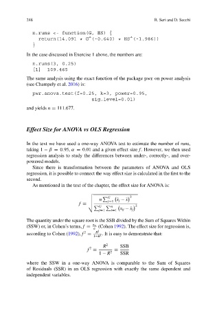
As mentioned in the text of the chapter, the effect size for ANOVA is:

v
u P G 2
n N x j Nx
u jD1
t
f D 2
P G P n
jD1 iD1 x ij Nx j
The quantity under the square root is the SSB divided by the Sum of Squares Within
m (Cohen 1992). The effect size for regression is,
(SSW) or, in Cohen’s terms, f D
2 R 2
1 R
according to Cohen (1992), f D 2 . It is easy to demonstrate that:
R 2 SSB
2
1 R SSR
f D 2 D
where the SSW in a one-way ANOVA is comparable to the Sum of Squares
of Residuals (SSR) in an OLS regression with exactly the same dependent and
independent variables.