Page 249 -

11 How Many Times Should One Run a Computational Simulation? 247

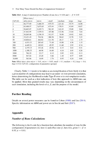
Table 11.4 A map of statistical power: Number of runs for ˛ D 0:01 and 1 ˇ D 0:95
Effect sizes f
CoP (G) ultra-micro micro small medium large huge
2 84,777.89 3,468.39 875.55 221.02 55.79 14.08
3 65,400.97 2,675.65 675.44 170.51 43.04 10.87
4 54,403.07 2,225.71 561.85 141.83 35.80 9.04
5 47,162.95 1,929.51 487.08 122.96 31.04 7.84
10 30,265.08 1,238.19 312.57 78.90 19.92 5.03
20 19,421.49 794.56 200.58 50.63 12.78 3.23
50 10,804.41 442.02 111.58 28.17 7.11 1.79
100 6,933.33 283.65 71.60 18.08 4.56 1.15
200 4,449.21 182.02 45.95 11.60 2.93 0.74
500 2,475.15 101.26 25.56 6.45 1.63 0.41
1000 1,588.33 64.98 16.40 4.14 1.05 0.26
3000 786.29 32.17 8.12 2.05 0.52 0.13
5000 567.02 23.20 5.86 1.48 0.37 0.09
10,000 363.86 14.89 3.76 0.95 0.24 0.06
Note. Effect sizes: ultra-micro D 0:01, micro D 0:05, small D 0:1, medium D 0:2, large D 0:4,
huge D 0:8.CoP (G): configuration of parameters (groups)

Clearly, Table 11.4 needs to be taken as an exemplification of how likely it is that
a given number of configurations may lead to an under- or over-powered simulation,
hence determining the likelihood to make Type-II error or to over-emphasize results.
The table can be used as a first indication of how this approach to ABM runs can
be applied. More fine grained results may vary depending on the circumstances of
each simulation, including the levels of ˛, ˇ, and the purpose of the model.

Further Reading

Details on several power measures can be found in Cohen (1988) and Liu (2014).
Specific information on ABM and power are in Secchi and Seri (2017).

Appendix

Number of Runs Calculations

The following is the R code for a function that calculates the number of runs for the

configuration of parameters (G, here G) and effect size (f, here ES), given 1 ˇ D
0:95, ˛ D 0:01: