Page 119 - Six Sigma Demystified

100 Six SigMa DemystifieD

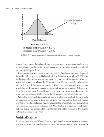
Figure 5.2 an improper use of confidence intervals to detect process changes.

value of the statistic based on the data, an assumed distribution (such as the
normal, Poisson, or binomial distribution), and a confidence level (usually 95
percent) (see Figure 5.2).
For example, the average error rate can be calculated over a six- month period
for a telemarketing process. If this calculation, based on a sample of 5,000 tele-
marketing calls, indicates an average process error rate of 3.4 percent, then the
lower and upper bounds on the 95 percent confidence interval can be calcu-
lated at 2.9 and 3.9 percent, respectively (based on techniques described later
in this book). If a current sample is taken and has an error rate of 3.8 percent,

then the current sample could have come from the same population as the
prior samples because it falls within the 95 percent confidence interval.
When these classical statistical methods of analysis are applied, the prior data
are assumed to be from a fixed population: The population does not change
over time. Fixed populations may be represented graphically by a distribution
curve such as that shown in Figure 5.2. Note that in this case a normal distri-
butional curve was assumed for convenience, as is often the case in hypothesis
tests and confidence intervals.

analytical Statistics

A process, however, is different from a population because it occurs over time.
In a process, variation may be due to causes that are persistent or to causes that