Page 171 - Six Sigma Demystified

152 Six SigMa DemystifieD

The total cycle time, the sum of the cycle times for the process steps, is
shown in Figure 7.1. The resulting distribution is nonnormal, which can be
verified using the normal probability plot and the Kolmogorov- Smirnov (K- S)
goodness- of- fit test. If the data are assumed to come from a controlled non-
normal process, the capability index indicates that the process will not meet the
requirements for a 45-hour cycle time.
The effect of cycle time reduction for each of the process steps then can be
evaluated. What is the effect of reducing the variation in step 1 by 50 percent?
How much will total cycle time be reduced if the average cycle time for step 2
is reduced to 5 hours? If it costs twice as much to reduce the variation in step
2, is the reduction in step 1 preferred? The effect of each of these scenarios can
be easily estimated using the simulation tool.
In a similar way, the effect of process variation on more complicated regres-
sion functions can be easily estimated. The effect of tightly controlling tempera-
ture on the consistency of product purity can be evaluated without first having
to implement an expensive temperature- control mechanism.
It should be clear that simulations offer a relatively simple and cost- effective
method of evaluating process improvement schemes. Since the simulation is a
direct reflection of the assumed model and its parameters, the results of the
simulation always must be verified in realistic process conditions. Regardless,
the cost of data acquisition is greatly reduced by the knowledge gained in the
process simulations.
Simulations allow the process flow to be easily revised “on paper” and evalu-
ated for flow, bottlenecks, and cycle times. These “what- if” scenarios save the
time and expense of actually changing the process to measure the effect. Once
the process is modeled, the before and after states can be compared easily for

resource allocation, costs, and scheduling issues.

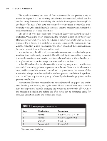
Table 7.1 Example Cycle Time Reduction
Step Distribution Parameters

1 Normal Mean = 12.1; SD = 1.9
2 Normal Mean = 7.3; SD = 0.5
3 Uniform Mean = 3
4 Exponential Mean = 5.1

SD = standard deviation.