Page 208 - Soil and water contamination, 2nd edition

Substance transport 195

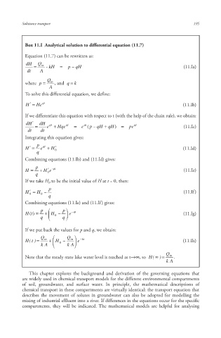
Box 11.I Analytical solution to differential equation (11.7)

Equation (11.7) can be rewritten as:
dH Q in
- kH p qH (11.Ia)
dt A
Q
where p in , and q k
A
To solve this differential equation, we define:
H He qt (11.Ib)

If we differentiate this equation with respect to t (with the help of the chain rule), we obtain:
d H dH qt qt qt qt
e Hqe e ( p qH qH ) pe (11.Ic)
dt dt
Integrating this equation gives:
p qt
H e H 0 (11.Id)
q
Combining equations (11.Ib) and (11.Id) gives:
p
H H 0 e -qt (11.Ie)
q
If we take H to be the initial value of H at t = 0, then:
0
p
H H 0 (11.If)
0
q
Combining equations (11.Ie) and (11.If) gives:
p p qt
H( t ) H 0 e (11.Ig)
q q

If we put back the values for p and q, we obtain:
Q in Q in kt
H ) t ( H 0 e (11.Ih)
k A k A
Q in
Note that the steady state lake water level is reached as t→∞, so H ( ) .
k A

This chapter explores the background and derivation of the governing equations that
are widely used in chemical transport models for the different environmental compartments
of soil, groundwater, and surface water. In principle, the mathematical descriptions of
chemical transport in these compartments are virtually identical: the transport equation that
describes the movement of solutes in groundwater can also be adopted for modelling the
mixing of industrial effluent into a river. If differences in the equations occur for the specific
compartments, they will be indicated. The mathematical models are helpful for analysing

10/1/2013 6:44:45 PM
Soil and Water.indd 207
Soil and Water.indd 207 10/1/2013 6:44:45 PM