Page 210 - Soil and water contamination, 2nd edition

Substance transport 197

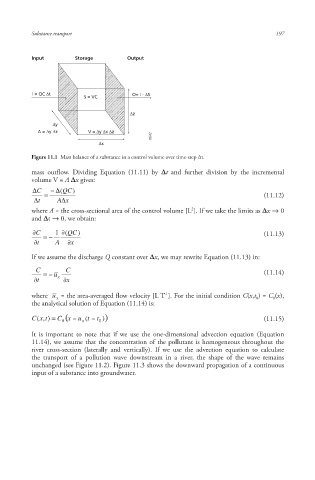
Input Storage Output

I = QC Δt O= I - ΔS
S = VC
Δz
Δy
A = Δy Δz V = Δy Δx Δz
6642
Δx
Figure 11.1 Mass balance of a substance in a control volume over time-step Δt.
mass outflow. Dividing Equation (11.11) by Δt and further division by the incremental
volume V = A Δx gives:
C ( QC)
(11.12)
t A x
2
where A = the cross-sectional area of the control volume [L ]. If we take the limits as Δx → 0
and Δt → 0, we obtain:
C 1 ( QC) (11.13)

t A x

If we assume the discharge Q constant over Δx, we may rewrite Equation (11.13) in:
C C
u x (11.14)
t x
-1
where u = the area-averaged flow velocity [L T ]. For the initial condition C(x,t ) = C (x),
x 0 0
the analytical solution of Equation (11.14) is:
(x ,t ) C 0 C u x (t t 0 ) x (11.15)

It is important to note that if we use the one-dimensional advection equation (Equation
11.14), we assume that the concentration of the pollutant is homogeneous throughout the
river cross-section (laterally and vertically). If we use the advection equation to calculate
the transport of a pollution wave downstream in a river, the shape of the wave remains
unchanged (see Figure 11.2). Figure 11.3 shows the downward propagation of a continuous
input of a substance into groundwater.

10/1/2013 6:44:48 PM
Soil and Water.indd 209 10/1/2013 6:44:48 PM
Soil and Water.indd 209