Page 219 - Soil and water contamination, 2nd edition

206 Soil and Water Contamination

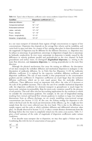
Table 11.1 Typical values of dispersion coefficient s under various conditions (adapted from Schnoor 1996)
Condition Dispersion coefficient (m s )
2
-1
Molecular diffusion 10 -9
-11
Compacted sediment 10 –10 -9
-9
Bioturbated sediment 10 – 10 -8
-6
Lakes – vertically 10 – 10 -3
-2
Rivers – laterally 10 – 10 1
Rivers – longitudinally 10 –10 3
1
3
Estuaries – longitudinally 10 –10 4
in a net mass transport of chemicals from regions of high concentrations to regions of low
concentrations. Dispersion thus depends on the average flow velocity and its variability, and
varies both in space and time. As a matter of fact, mixing takes place in three dimensions and
the magnitude of dispersion may be different for the different directions, i.e. dispersion may
be subject to anisotropy . In groundwater, anisotropy in dispersion is largely due to anisotropy
in hydraulic conductivity . In river water, anisotropy in dispersion is mainly caused by the
differences in velocity gradients parallel and perpendicular to the river channel. In both
groundwater and surface water, we distinguish longitudinal dispersion, i.e. mixing in the
main flow direction, and transverse dispersion , i.e. mixing perpendicular to the main flow
direction.
Although the physical mechanisms that cause the mixing are different, the description
of net mass transport by turbulent diffusion and mechanical dispersion is analogous to the
description of molecular diffusion . So, in Fick’s first law (Equation 11.18) for molecular
diffusion, coefficient D is replaced by the respective turbulent diffusion coefficient and
dispersion coefficient . The rate of mass transfer is thus proportional to the concentration
gradient and the coefficient D. Dispersion coefficients are much larger than the turbulent
diffusion coefficients, which are in turn much greater than the molecular diffusion
coefficients. These differences reveal an important scale effect: the value of D increases as
the scale of the problem increases. This is also the case if we consider mechanical dispersion
only: the dispersion coefficient for chemical transport in groundwater is much larger for
macro-scale variations in permeability than for micro-scale variations caused by the presence
of soil particles. This scale effect also has far-reaching implications for the resolution at which
we consider the concentration gradients. For example, in the case of longitudinal mixing
resulting from vertical and lateral flow velocity gradients in medium to large river channels
downstream from an effluent discharge, we are mostly modelling cross-sectional average
concentrations (see Section 11.3.3). In this case, the Fickian analogy for dispersion is not
valid at the local scale for the reach just downstream of the effluent, e.g. for a single one litre
sample from the river water collected near the river bank. This is due to the difference in
sample support and the scale at which turbulent diffusion and differential advection takes
place. As already observed in Section 11.2.2, it takes a certain distance downstream from the
discharge before the river water is completely mixed over the entire cross-section. Table 11.1
gives a brief summary of the order of magnitude of dispersion coefficients under various
conditions.
If we describe mass transport due to dispersion , we may thus apply a Fickian type law.
Combining this with the law of conservation of mass gives:
C J
(11.19)
t x

10/1/2013 6:44:53 PM
Soil and Water.indd 218 10/1/2013 6:44:53 PM
Soil and Water.indd 218