Page 222 - Soil and water contamination, 2nd edition

Substance transport 209

t=0 Centre of mass at times t , t , and t
x=0 1 2 3
t 1 t 2 t 3

L 1

L 2 x - direction

L 3

max
C at t 1

Concentration C at t 2 C at t 3
max
max

0.61 C max
2σ
6642
0 L 1 L 2 L 3
Distance (x)

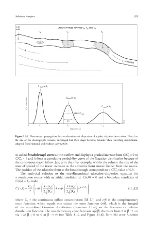
Figure 11.6 Downstream propagation due to advection and dispersion of a pulse injection into a river . Note that
the size of the chemographs remains unchanged but their shape becomes broader while travelling downstream.
Adapted from Hemond and Fechner-Levy (2000).

so-called breakthrough curve at the outflow end displays a gradual increase from C/C = 0 to
0
C/C = 1 and follows a cumulative probability curve of the Gaussian distribution because of
0
the continuous tracer inflow. Just as in the river example, within the column the size of the
zone of spread of the tracer increases as the advective front moves further from the source.
The position of the advective front at the breakthrough corresponds to a C/C value of 0.5.
0
The analytical solution to the one-dimensional advection–dispersion equation for
a continuous source with an initial condition of C(x,0) = 0 and a boundary condition of
C(0,t) = C reads:
0
C x u t x u t
C( x, t) 0 erfc x erfc x e u x x / D x (11.32)
2 2 D x t 2 D x t

-3
where C = the continuous inflow concentration [M L ] and erfc is the complementary
0
error function , which equals one minus the error function (erf), which is the integral
of the normalised Gaussian distribution (Equation 11.26) or the Gaussian cumulative
distribution function. The complementary error function erfc(β) decreases from 2 at β → -∞
via 1 at β = 0 to 0 at β → ∞ (see Table 11.2 and Figure 11.8). Both the error function

10/1/2013 6:44:56 PM
Soil and Water.indd 221 10/1/2013 6:44:56 PM
Soil and Water.indd 221