Page 37 - Soil and water contamination, 2nd edition

24 Soil and Water Contamination

80

70 1.2 1.0
C s = 2.0 C w C s = 2.0 C w
60
C s = 50 x 1.0 C w
50 1 + 1.0 C w
C s (mg/kg) 40 C s = 50 x 0.1 C w

30 1 + 0.1 C w

0,7
20 C s = 2.0 C w
10
6642 0
0 5 10 15 20 25 30 35 40 45 50
C w (mg/l)

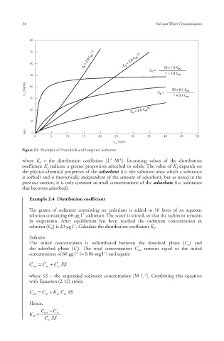
Figure 2.1 Examples of Freundlich and Langmuir isotherms .
-1
3
where K = the distribution coefficient [L M ]. Increasing values of the distribution
d
coefficient K indicate a greater proportion adsorbed to solids. The value of K depends on
d d
the physico-chemical properties of the adsorbent (i.e. the substrate onto which a substance
is sorbed) and is theoretically independent of the amount of adsorbent, but as noted in the
previous section, it is only constant at small concentrations of the adsorbate (i.e. substance
that becomes adsorbed).
Example 2.4 Distribution coefficient
Ten grams of sediment containing no cadmium is added to 10 litres of an aqueous
-1
solution containing 60 μg l cadmium. The water is stirred, so that the sediment remains
in suspension. After equilibrium has been reached the cadmium concentration in
-1

solution (C ) is 20 μg l . Calculate the distribution coefficient K .
w d
Solution
The initial concentration is redistributed between the dissolved phase (C ) and
w

the adsorbed phase (C ). The total concentration C remains equal to the initial
s
tot
-1
-1
concentration of 60 μg l (= 0.06 mg l ) and equals:
C tot C C s SS
w
-3
where SS = the suspended sediment concentration [M L ]. Combining this equation
with Equation (2.12) yields:
C C K C SS
tot w d w
Hence,
C tot C w
K
d
C w SS

10/1/2013 6:44:11 PM
Soil and Water.indd 36
Soil and Water.indd 36 10/1/2013 6:44:11 PM