Page 192 - Statistics II for Dummies

176 Part III: Analyzing Variance with ANOVA

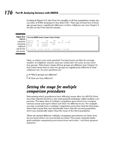
Looking at Figure 10-2, the F-test for equality of all four population means has
a p-value of 0.000, meaning it’s less than 0.001. That says at least two of these
age groups have a significant difference in their cellphone use (see Chapter 9
for info on the F-test and its results).

Figure 10-2: One-way ANOVA: Group 1, Group 2, Group 3, Group 4
ANOVA
Source DF SS MS F P
results for
Factor 3 2416010 805337 204.13 0.000
comparing Error 36 142030 3945
cellphone Total 39 2558040
use for four S = 62.81 R–Sq = 94.5% R–Sq(adj) = 93.99%
age groups.

Okay, so what’s your next question? You just found out that the average
number of cellphone minutes used per month isn’t the same across these
four groups. This doesn’t mean all four groups are different (see Chapter 9),
but it does mean that at least two groups are significantly different in their
cellphone use. So your questions are
✓ Which groups are different?
✓ How are they different?

Setting the stage for multiple

comparison procedures

Determining which populations have differing means after the ANOVA F-test
has been rejected involves a new data-analysis technique called multiple com-
parisons. The basic idea of multiple comparison procedures is to compare
various means and report where and what the differences are. For example,
you may conclude from a multiple comparison procedure that the first popu-
lation had a mean that was statistically lower than the second population,
but it was statistically higher than the mean of the third population.

There are myriad different multiple comparison procedures out there; how
do you know which one you should use when? Two basic elements distin-
guish multiple comparison procedures from each other. I call them purpose
and price.

16_466469-ch10.indd 176 7/24/09 9:41:32 AM