Page 77 - Statistics II for Dummies

Chapter 4: Getting in Line with Simple Linear Regression 61

that does this for you (computers use it in their calculations). Formulas also
exist for finding the slope and y-intercept of the best-fitting line by hand. The
best-fitting line based on your data is y = a + bx, where a estimates α and b
estimates β from the true model. (You can find those formulas in your Stats I
text or in Statistics For Dummies.)
To run a linear regression analysis in Minitab, go to Stat>Regression>
Regression. Highlight the response (y) variable in the left-hand box, and click
Select. The variable shows up in the Response Variable box. Then highlight
your explanatory (x) variable, and click Select. This variable shows up in the
Predictor Variable box. Click OK.

The equation of the line that best describes the relationship between average
textbook weight and average student weight is y = 3.69 + 0.113x, where x
is the average student weight for that grade, and y is the average textbook
weight. Figure 4-2 shows the Minitab output of this analysis.

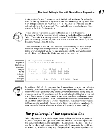
The regression equation is
Figure 4-2: textbook wt = 3.69 + 0.113 student wt
Simple linear
regression
analysis Predictor Coef SE Coef T P
for the Constant 3.694 1.395 2.65 0.024
textbook- student wt 0.11337 0.01456 7.78 0.000
weight
example. S = 1.51341 R-Sq = 85.8% R-Sq(adj) = 84.4%

By writing y = 3.69 + 0.113x, you mean that this equation represents your estimated
value of y, given the value of x that you observe with your data. Statisticians tech-
y
nically write this equation by using a caret (or hat as statisticians call it), like ˆ, so
everyone can know it’s an estimate, not the actual value of y. This y-hat is your esti-
mate of the average value of y over the long term, based on the observed values
of x. However, in many Stats I texts, the hat is left off because statisticians have
an unwritten understanding as to what y represents. This issue comes up again
in Chapters 5 through 8. (By the way, if you think y-hat is a funny term here, it’s
even funnier in Mexico, where statisticians call it y-sombrero — no kidding!)

The y-intercept of the regression line

Selected parts of that Minitab output shown in Figure 4-2 are of importance
to you at this point. First, you can see that under the Coef column you have
the numerical values on the right side of the equation of the line — in other
words, the slope and y-intercept. The number 3.69 represents the coefficient
of “Constant,” which is a fancy way of saying that’s the y-intercept (because

09_466469-ch04.indd 61 7/24/09 10:20:36 AM