Page 84 - Statistics II for Dummies

68 Part II: Using Different Types of Regression to Make Predictions

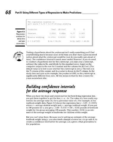
The regression equation is
quiz score = 3.29 + 0.179 minutes studying

Predictor Coef SE Coef T P
Figure 4-3:
Regression Constant 3.2931 0.4864 6.77 0.000
analysis for Minutes studying 0.17931 0.02103 8.53 0.000
study time
and quiz S = 0.877153 R-Sq = 90.1% R-Sq (adj) = 88.8%
score data.

Testing a hypothesis about the y-intercept isn’t really something you’ll find
yourself doing much because most of the time you don’t have a preconceived
notion about what the y-intercept would be (nor do you really care ahead of
time). The confidence interval is much more useful. However, if you do need
to conduct a hypothesis test for the y-intercept, you take your y-intercept,
subtract the value in Ho, and divide by the standard error, found on the
computer output in the row for Constant and the column for SE Coef. (The
default value is to test to see whether the y-intercept is zero.) The test is in
the T column of the output, and its p-value is shown in the P column. In the
study time and quiz score example, the p-value is 0.000, so the y-intercept is
significantly different from zero. All this means is that the line crosses the
y-axis somewhere else.

Building confidence intervals

for the average response

When you have the slope and y-intercept for the best-fitting regression line,
you put them together to get the line y = a + bx. The value of y here really rep-
resents the average value of y for a particular value of x. For example, in the
textbook-weight data, Figure 4-2 shows the regression line y = 3.69 + 0.11337x
where x = average student weight and y = average textbook weight. If you put
in 100 pounds for x, you get y = 3.69 + 0.1137 * 100 = 15.02 pounds of textbook
weight for the group averaging 100 pounds. This number, 15.02, is an esti-
mate of the average weight of textbooks for children of this weight.

But you can’t stop there. Because you’re getting an estimate of the average
textbook weight using y, you also need a margin of error for y to go with it, to
create a confidence interval for the average y at a given x that generalizes to
the population.

09_466469-ch04.indd 68 7/24/09 10:20:38 AM