Page 101 - Statistics and Data Analysis in Geology

Analysis of Sequences of Data

The same reasoning can be applied to determine the probability of any lithology
two steps hence, from any starting lithology. However, all of the various sequences
do not have to be worked out individually, because the process of multiplying and
summing is exactly that used for matrix multiplication. If the transition probability
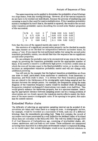
matrix is multiplied by itself (that is, the matrix is squared), the result is the second-
order transition probability matrix describing the second-order Markov properties
of the succession:

0.78 0 0.22 0 0.64 0.02 0.31 0.02
0 0.71 0.29 0 1' = [ 0.05 0.52 0.39 0.03 1
0.18 0.07 0.64 0.11 0.26 0.09 0.54 0.11
0 0 0.60 0.40 0.11 0.04 0.62 0.23

Note that the rows of the squared matrix also sum to 100%.
The existence of a significant second-order property can be checked in exactly
the same manner as we checked for independence between successive states, by
using a x2 test. If you repeat the test performed earlier, but using the second-order
transition probability matrix, you should find that the sequence has no significant
second-order properties.
We can estimate the probable state to be encountered at any step in the future
simply by powering the transition probability matrix the appropriate number of
times. If the matrix is raised to a sufficiently high power, it reaches a stable state in
which the rows all become equal to the fixed probability vector, or in other words,
becomes an independent transition probability matrix and will not change with
additional powering.
You will note in the example that the highest transition probabilities are from
one state to itself, particularly from sandstone to sandstone, from limestone to
limestone, and from shale to shale. It is obvious that these transition probabili-
ties are related to the thicknesses of the stratigraphic units being sampled and the
distance between the sample points. For example, the frequencies along the main
diagonal of the transition frequency matrix would be doubled while off-diagonal
frequencies remained unchanged if observations were made every half-foot. This
would greatly enhance the Markovian property, but in a specious manner. Select-
ing the appropriate distance between sampling points can be a vexing problem; if
observations are too closely spaced, the transition matrix reflects mainly the thick-
ness of the more massive stratigraphic units. If the spacing is too great, thin units
may be entirely missed.

Embedded Markov chains

The difficulty of selecting an appropriate sampling interval can be avoided if ob-
servations are taken only when there is a change in state. A stratigraphic section,
for example, would be recorded as a succession of beds, each one of a different
lithology than the immediately preceding bed. Table 4-4 contains the record of
successive rock types penetrated by a well drilled in the Midland Valley of Scotland
(these data are contained in file MIDLAND.TXT). The well was drilled through 1600
ft of Coal Measures of Carboniferous age, consisting of interbedded shales, silt-
stones, sandstones, and coal beds or root zones. These sediments are interpreted
as having been deposited in a delta plain environment subject to repeated flooding,
so we would expect that certain lithologies would occur in preferred relations to

173